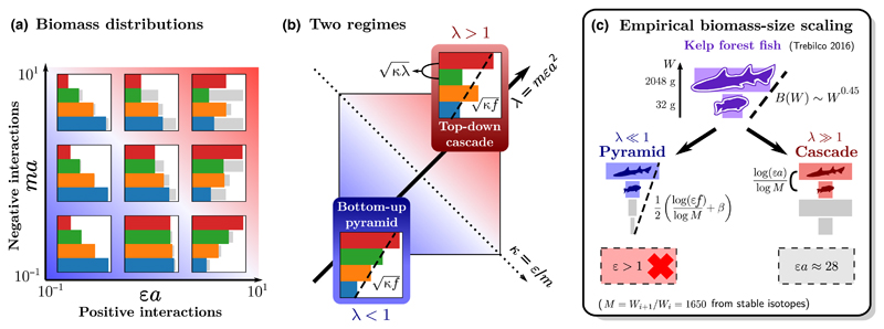
Figure 3.

Theoretical map of equilibrium biomass patterns in a food chain, and application to an empirical puzzle. The parameters (defined in Box 1) are predator–prey metabolic ratio m, conversion efficiency ε and the strength of interactions a relative to self-interaction. Results are illustrated for a four-level chain with negligible metabolic losses ρ≪1 (other examples in Supporting Information). (a) Biomass distribution. For each trophic level, a coloured bar represents its equilibrium biomass (in log scale), and a grey bar represents the amount of biomass lost to its predator, reflecting the intensity of top-down control. (b) Two parameter regimes define the shape of the biomass distribution. The main diagonal λ = mϵa² distinguishes the region of bottom-up control λ < 1 with pyramids (both regular and inverted), from the region of top-down control λ > 1 with cascade (alternating) patterns. The other diagonal κ = ε/m affects the top-heaviness of the biomass distribution, as the global slope of the distribution is given by $B_{i+1}/B_i~\sqrt{\kappa f}.$ The fraction f of production lost to consumers is given by (16). In cascade patterns, low-biomass and high-biomass levels i and i+1 alternate, with $B_{i+1}/B_i~\sqrt{\kappa \lambda }=\mathit{ϵ}a$ (larger than the global slope, which still holds between levels B_i+1 and B_i−1). (c) Identifying trophic structure from data. Given the biomass per trophic level and the mass ratio M between levels, we can compute the total biomass in each body size class W. Fish in kelp forests exhibit a top-heavy (positive) scaling B(W)~W^0.45 (Trebilco et al. 2016). We show in main text that this scaling cannot hold across multiple trophic levels, except for an unphysical value of conversion efficiency ε > 1 in formula (18). It may, however, be found between two adjacent levels under strong top-down control (19).