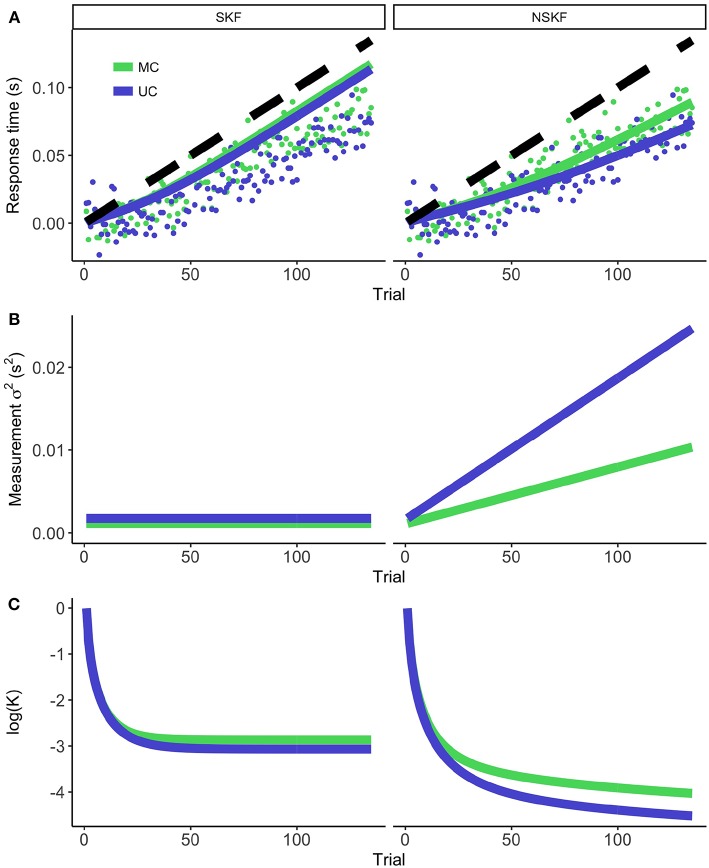
Figure 3.
The modeling results for the stationary (left) and non-stationary (right) Kalman filter. (A) The average response times (dots) and model prediction (colored lines) for the MC and UC condition. The black dashed line represents the temporal perturbation of the action during the experiment. (B) The measurement noise as calculated from equation 7 (SKF) and 8 (NSKF). (C) The resulting log(Kalman Gain).

