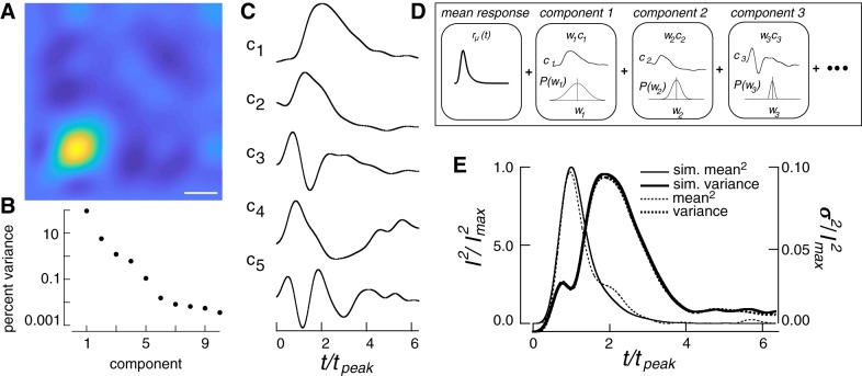
Fig. 4.

Using the response covariance to simulate single-photon responses. A: covariance matrix of the single-photon response. Time of flash is the lower left vertex. Scale bar, 300 ms. B: percent of the total variance captured by each eigenvector (c_i) of the covariance matrix in A. C: the five components used to simulate single-photon responses. D: generation of response from components, as in Eq. 7. A simulated response was generated by combining single-photon responses with two components of dark noise. Each single-photon response was generated as a sum of temporal components corresponding to eigenvectors of the corrected covariance matrix. Each component was weighted by a coefficient drawn from a Gaussian distribution with variance corresponding to the appropriate eigenvalue. See Eq. 7 and associated text for definitions of parameters. E: time-dependent variance and the squared mean single-photon response of the model compared with those measured experimentally. I², mean squared response; I²_max, peak response squared; r_m, mean single photon response; sim., simulated; t, time; t_peak, time to peak.