Figure 8.

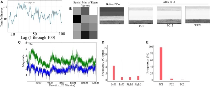
CTE - (A) Grand-average of TE values for Lag = 1, …, 100 (i.e., up to 10 s of lag, considering the sampling rate of 10.0 Hz in our device). Maximum TE was at Lag = 30 (equivalent to time = 3.0 s) (B) Sample spatial map of eigenvectors by PCA-based SBF attenuation algorithm along with a sample participant's PFC time series (in matrix forms for better visualization purpose) before and after application of PC1, PC12, and PC123 components. Distinctive effect of these components on participant's PFC time series is evident in this subplot. All matrices are scaled within [0, 1] interval for ease of comparison. (C) Sample SBF (blue) and the corresponding IC1 component computed by ICA-based SBF attenuation algorithm (blue). The depicted IC1 component pertains to the case in which Right₁ was selected as component with highest coefficient of spatial uniformity. (D) Frequency of selected channels as a component with highest coefficient of spatial uniformity by ICA-based SBF attenuation algorithm for CTE dataset. (E) Percentages of the variance-explained by each of the principal components (i.e., PC1, PC12, PC123) of PCA-based SBF attenuation algorithm for CTE dataset.