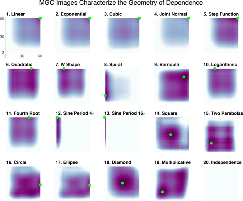
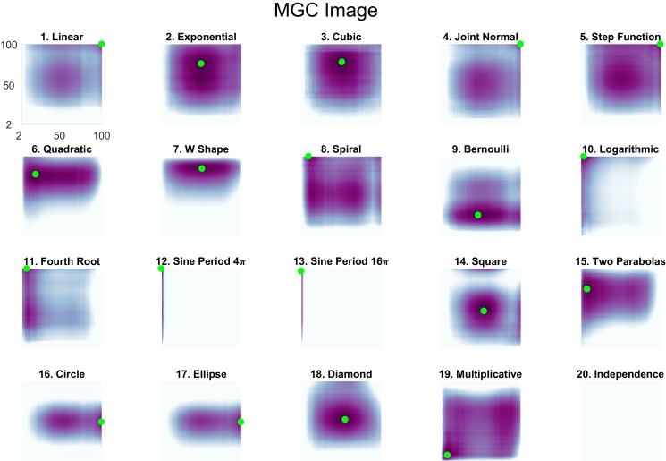
Figure 3. The Mgc-Map characterizes the geometry of the dependence function.

For each of the 20 panels, the abscissa and ordinate denote the number of neighbors for $X$ and $Y$, respectively, and the color denotes the magnitude of each local correlation. For each simulation, the sample size is 60, and both $X$ and $Y$ are one-dimensional. Each dependency has a different Mgc-Map characterizing the geometry of dependence, and the optimal scale is shown in green. In linear or close-to-linear relationships (first row), the optimal scale is global, that is the green dot is in the top right corner. Otherwise the optimal scale is non-global, which holds for the remaining dependencies. Moreover, similar dependencies often share similar Mgc-Maps and similar optimal scales, such as (10) logarithmic and (11) fourth root, the trigonometric functions in (12) and (13 , 16) circle and (17) ellipse, and (14) square and (18) diamond. The Mgc-Maps for high-dimensional simulations are provided in Figure 3—figure supplement 1.

Figure 3—figure supplement 1. The Mgc-Map for the 20 panels for high-dimensional dependencies.

For each simulation, the sample size is 100, and the dimension is selected as the dimension such that Mgc has a testing power above 0.5. It has similar behavior and interpretation as the one-dimensional power maps in Figure 3, that is the linear relationships optimal scales are global, and similar dependencies share similar Mgc-Maps.