Black soldier fly larvae feed by forming a fountain around food

Abstract

The black soldier fly is a non-pest insect of interest to the sustainability community due to the high eating rates of its edible larvae. When found on carcases or piles of rotting fruit, this larva often outcompetes other species of scavengers for food. In this combined experimental and theoretical study, we elucidate the mechanism by which groups of black soldier fly larvae can eat so quickly. We use time-lapse videography and particle image velocimetry to investigate feeding by black soldier fly larvae. Individually, larvae eat in 5 min bursts, for 44% of the time, they are near food. This results in their forming roadblocks around the food, reducing the rate that food is consumed. To overcome these limitations, larvae push each other away from the food source, resulting in the formation of a fountain of larvae. Larvae crawl towards the food from below, feed and then are expelled on the top layer. This self-propagating flow pushes away potential roadblocks, thereby increasing eating rate. We present mathematical models for the rate of eating, incorporating flow rates measured from our experiments.

1. Introduction

Humans produce 1.3 billion tons of food waste per year [1]. Raising black soldier fly larvae, Hermetia illucens, is one promising method to deal with this waste. Larva farmers raise thousands of larvae together in bins and feed them food waste. A single larva is shown in figure 1a. Figure 1b and electronic supplementary material, video S1, show a swarm of larvae consuming a 16-inch pizza in 2 h. At the end of their lives, the larvae are used as a sustainable feed source for chickens, fish and other livestock animals [2,3]. When farming larvae, maximizing eating rate is desired so that the larvae can grow as quickly as possible. While past studies of larva feeding give estimates for their eating rate [2], little detail is given on the number of individuals. The goal of this study is to determine the mechanism by which groups of larvae feed.

Figure 1.

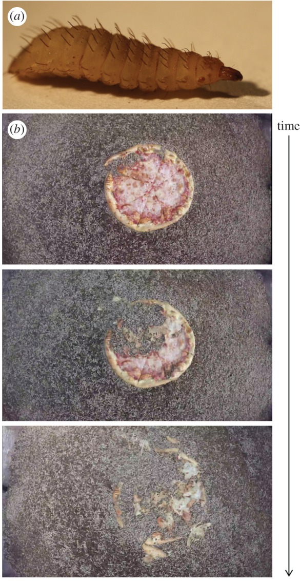
(a) The black soldier fly larva shown is 14 mm long and weighs 0.1 g. (b) A group of larvae consumes a 40 cm diameter pizza in 2 h. The motion of the pizza crust and cheese away from the centre indicates that the motion of larvae is correlated with their neighbours. These images are courtesy of Grubbly Farms. (Online version in colour.)

Although there has been much work done on collective animal movement [4], little is known about collective feeding. Such feeding behaviour is universal because migratory animals often feed together. This is the case for swarms of locusts, which can destroy fields of crops, or piranha shoals, which can remove the flesh from animals in minutes. In fact, high feeding rates are used to accomplish tasks that would be difficult to do otherwise: dermestid beetles eat dead flesh so thoroughly that they are used by museums to clean bones, but how their feeding rate depends on the number of beetles remains unknown [5]. Comparatively more work has been done on the feeding of livestock, due to its importance to agriculture. However, it has been investigated for specific cases that are difficult to generalize—for example, the behaviour of growing pigs in single-space feeders or the social consequences of moving cows between groups [6,7]. Moreover, experiments with cows and pigs necessarily involve fewer numbers of individuals than the group feeding of insects.

In order to understand how larvae feed so quickly, one of the methods we use in this study is the visualization of their collective movement. Tracking individuals in three-dimensional swarms has been done with hundreds of birds [8,9]. The larvae are challenging to visualize because the individuals are in closer proximity than birds in flocks or fish in schools. Rather than visualize the motion of larvae inside the opaque aggregation, we visualize it with two-dimensional imaging from the top and bottom and use particle image velocimetry (PIV) to analyse their flows and infer motion inside the aggregation. Typical PIV analysis uses tracer particles in the fluid to be imaged. The positions of the tracer particles in frames of camera images are correlated to find velocity vectors between frames. In active matter research, the technique is adapted so that the organism being studied is used as the tracer particle. PIV has been successfully used with bacteria and with microtubule networks [10,11]. Bacteria swim in a fluid or atop a substrate and two-dimensional layers have been previously visualized. We adopt similar methods and film the top and bottom of the larva aggregation.

In this study, we investigate how larvae consume food so quickly in large groups. We proceed in §2 by presenting our experimental methods for studying larva feeding, followed by our mathematical modelling methods in §3. We then present our experimental results, including observations of single larva feeding, PIV tracking of larva groups, and measurements of eating rate in §4. In §5, we discuss the implications of our work, and we conclude in §6.

2. Material and methods

2.1. Larva care

Black soldier fly larvae are obtained from Grubbly Farms at 8–12 days old, and weighing about 0.1 g. They are starved for 24 h before any experiments. On the remaining days, larvae in the individual eating rate experiments and PIV experiments are fed chicken feed; larvae in group feeding rate experiments are fed leftover fruit pulp from smoothies.

The large numbers of larvae in PIV trials are counted by measuring their volume. To begin, we weigh 100 larvae using an analytical balance to infer that the mass of a single larva is 0.09 g. We use the mass of one larva to measure out 1000 larvae, again on an analytical balance. The larvae are placed in a 250 ml beaker, where we immediately measure their volume so they do not have time to actively settle. We find that 1000 larvae have a volume of V_total = 175 ml. If every larva has an average length L = 13.7 mm, width w = 4.3 mm and height h = 3.2 mm, then its volume, that of an ellipsoid, is V_larva = (π/6) whL ∼ 0.1 cm³. The average packing fraction of larvae is therefore 1000V_larva/V_total = 0.56. The maximum packing of ellipsoids is 0.735, so larvae are much less densely packed than they could be if they were allowed to settle [12]. Using this packing fraction, we proceed by using volume to measure out 3000, 5000 and 10 000 larvae in increments of 175 ml of larvae.

In group feeding trials, the number of larvae in an aggregation is estimated by weighing the aggregation with an analytical balance (for 1000 or fewer larvae) or a Smart Weigh ACE110 Digital Scale (for more than 1000 larvae).

2.2. Feeding by a single larva

The mouth of a dead larva is photographed with a BK PLUS lab system by Dun, Inc. We determine the chemical composition of the mouth and head by examining a dead larva in a scanning electron microscope (LEO 1530 by Carl Zeiss, AG, Oberkochen, Germany) with an attached energy dispersive X-ray spectrometer (Oxford Instruments, Abingdon, UK).

High speed videos are taken with a Phantom Miro M110 high speed camera at 500 frames per second. The larva’s mouth is pushed through a hole cut in a piece of tape to hold it in place during filming. We track the positions of the maxillae in a video generated from the high-speed video at 150 frames per second using the free software Tracker from physlets.org. The length of the mandibular brush, L_brush = 0.38 mm, is used for scale. There is an error due to the head movement of the larva, but this displacement is small compared to the movement of the maxillae.

To measure how often larvae feed, we perform experiments with single larvae. We place each of 10 larvae into 10 separate 10 cm diameter petri dishes and fed them with a 0.2 g lump of food in the centre of the dish. The food is a mixture of 50% chicken feed (Southern States Layer and Breeder) and 50% water by volume. This food stays in a single lump without leaking unless a larva breaks it, facilitating our tracking if a larva makes contact and is eating. We film a top view of the larvae with a Sony handycam (Model HDR-XR200V) for over an hour, and watch the videos afterward to mark the durations that the larvae remain in contact with the food, which we assume are the durations that the larvae feed. Fluorescent ceiling lamps are used to light the half of the laboratory that trials are not occurring in, indirectly lighting the larvae and not disturbing their feeding.

Throughout this study, we continue to use Sony handycams for all filming except high speed, but we will vary the food and lighting.

2.3. Particle image velocimetry of a group of larvae

A specially constructed apparatus is used to perform PIV on groups of larvae (figure 2a). A 10-gallon fish tank is set up on a metal cart with cameras mounted both above and underneath the tank. Fluorescent ceiling lamps illuminate the top view. To illuminate the bottom view, we point two LED lamps (Visual Instrumentation Corporation, Model 900420 W) from the side. The lamps are covered in thin packaging foam and red cellophane because the lighting in this spectrum is less disruptive to insects [13]. To commence experiments, half of an orange slice (weighing 12 g) is pushed through a toothpick glued upright in the centre of the tank. The orange slice rind is peeled, but its walls are left intact so that it remains attached to the stick during feeding.

Figure 2.

(a) Set-up of particle image velocimetry experiment. Larvae are placed in a 10 gallon aquarium with cameras filming the top and bottom. (b) Sample instantaneous vectors from a top view of larvae around food. The vectors do not point to any mean flows, showing the need for averaging. (Online version in colour.)

Larvae aggregate around the orange as they eat it. We use PIV to determine the flow properties of the larva aggregation. Within the aggregation of larvae around food, we define a ‘mixing region’ as the area around the orange where the average velocity of larvae is greater than a threshold of 0.125 mm s⁻¹, or 1/16th the speed of a free larva. The mixing region is characterized by an inflow of larvae on the bottom layer and an outflow of larvae on the top layer, indicating that larvae form a coherent flow around food. Many of our calculations will refer to the velocity and size of this mixing region.

We do two types of experiments: an experiment with both a top and bottom view, and then experiments with varying numbers of larvae with a top view only. Performing analysis on both top and bottom view is time consuming, so the bottom view is performed sparingly. In the top and bottom views, 600 ml of larvae (approximately 3500 larvae) are placed in the tank and eat an orange slice as they are filmed. For each video, 1 h of footage is filmed. One frame per second of the resulting video is extracted from the top view, and one frame per 5 s of the video is extracted from the bottom view. Larvae on the bottom are jammed by the surrounding larvae and move slower than the ones on top. Larvae on the top view move faster, but less frequently, than larvae on the bottom view. Consequently, a longer time between frames is needed on the bottom view. Frames are extracted using the free software, Video to JPG Converter (www.dvdvideosoft.com).

Digitization and data extraction from the images are accomplished with Matlab. We write a script to crop raw images and convert them to white larvae on a black background. PIVlab [14,15] is used to measure the velocity fields between each pair of consecutive frames. A mask is drawn on top of the orange slice to avoid analysing that area. The interrogation windows, in which particle positions are correlated, decrease in size from 64 pixels to 32 pixels in two passes of analysis. Sample instantaneous vectors are shown in figure 2b. For the experiment filmed from top and bottom, the feeding is not analysed for the first 500 s, since the feeding is in a transient state. After this transient, the following 2000 s are analysed, during which the experiment is in steady state. We validate our PIV analysis by randomly reshuffling frames from 500 to 2500 s in the top view of this experiment: the resulting vector field after averaging, shown in electronic supplementary material, figure S1, shows the absence of a mixing region, as expected. This confirms that the resulting mixing region is not an artefact of our analysis.

For the single trial with a top and bottom view, the mixing region is not clearly above a particular threshold. This is likely caused by the bottom lighting disturbing the behaviour of the larvae. Instead, we estimate the mixing region by measuring its area within PIVlab to be about 80 cm² for the top view and 60 cm² for the bottom view (including the orange). We then draw this mask around the mixing region in the top and bottom views to determine the average velocity magnitude, divergence and vorticity.

In our trials with multiple group sizes, we perform top view PIV experiments with 500, 1000, 3000, 5000 and 10 000 larvae. Since larvae can only enter the mixing region from the top or bottom layer, the number of larvae leaving the food on the top view must be equal to the number of larvae coming in to eat on the bottom view. Thus, the top view is sufficient to calculate both the flow rate of larvae away from and towards food. The top view yields more consistent results because the bottom view lighting disturbs larva feeding. With fewer than 500 larvae in the container, the mixing region is too small for PIV analysis, so the analysis starts with 500 larvae. Only fluorescent ceiling lamps are used in these experiments. Only 35 min of the footage is filmed in these cases. 1500 s of motion are averaged, starting at 500 s. In PIV analysis, to reduce artefacts, a maximum possible velocity is set to 10 mm s⁻¹, or five times the speed of a free larva. The average vector fields are saved for further analysis as described in §2.4.

2.4. Measuring flow rate from particle image velocimetry

We define the rate of outflow of larvae as the number of larvae leaving the food per minute on the top layer of the mixing region. By conservation of mass at steady state, this flow rate is necessarily equal to the larvae entering the food below. To estimate the flow rate of larvae for mixing regions with 500–10 000 larvae, we calculate the flux from the boundary as determined by Matlab. Thus, Q, the number of larvae leaving per minute, may be written

$$Q=\frac{1}{V_{\mathrm{larva}}}\sum _{\mathrm{boundary}}(\mathbf{v}\cdot \mathbf{n})\hspace{0.17em}\text{d}A,$$ 2.1

where v is the velocity vector at each point, n is the normal to the boundary segment at that point, dA is the length of the segment multiplied by the layer depth (the height h of a larva, 3.2 mm) and V_larva ∼ 0.1 ml is the volume of a larva. The points making up the circumference of the mixing region are discretized into segments with length 5 ± 1 mm. The relationship between the number of larvae and flow rate is shown in figure 3f. We model this trend using a linear best fit for 1000 to 10 000 larvae:

$$Q=aN+b$$ 2.2

where a and b are coefficients and N is the number of larvae. To ensure that our velocity vectors calculated for 1500 s are meaningful, we recalculate the average vector fields with 1000 s duration and 500 s duration. We compare these average velocity fields for the 1000–10 000 larva trials. We find that the flow rate of larvae changes by a maximum 8 larvae per minute with averaging over 1000 s and maximum 11 larvae per minute with averaging over 500 s. Since Q is of the order of 50 larvae per minute for 1000 larvae and 100 larvae per minute for 3000 to 10 000 larvae, we are reassured that the flow rates are repeatable measurements.

Figure 3.

Images of the larvae and food after 33 min next to the corresponding time-averaged velocity fields, with the mixing region selected. (a) 500 larvae, (b) 1000 larvae, (c) 3000 larvae, (d) 5000 larvae and (e) 10 000 larvae. (f) The relationship between number of larvae and their flow rate. (Online version in colour.)

2.5. Measuring group eating rates

We measure larva eating rates by feeding pieces of orange slices weighing 6–18 g to larvae. Different containers are used for different numbers of larvae tested. Filming is done under red light to avoid disturbing the larvae. Groups of larvae numbering 500 and fewer are placed into plastic drink cups as shown in figure 4a. Groups of 1000–3000 larvae are placed into 1 l beakers. Groups of 5000–10 000 larvae are placed into containers (34.6 cm × 21 cm × 12.4 cm plastic Sterilite) while groups of 15 000–30 000 are placed in larger containers (42.9 cm × 29.2 cm × 23.5 cm plastic Sterilite). The test with 58 000 larvae is done in a concrete mixing tub (86.4 cm × 58.4 cm × 17.8 cm).

Figure 4.

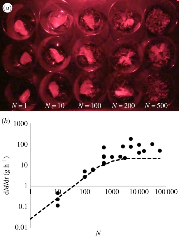
(a) Experimental set-up to measure the eating rate of larvae. (b) Relationship between eating rate and number of larvae. Dots are experimental data points and dashed line is the model. (Online version in colour.)

Experiments are performed throughout the summer and autumn of 2016, in an indoor laboratory or an open-air warehouse. All experiments involve feeding an orange slice to larvae of various group sizes, and then weighing it (Mettler Toledo Classic Plus analytical balance) to determine the amount eaten. The duration of eating is varied from 5 to 30 min, depending on the size of the group. Larger numbers of larvae eat faster, so necessitate a shorter experimental duration; smaller numbers of larvae required longer times in order to obtain an accurate estimate of the mass eaten. The slice was weighed after 30 min for aggregations of 200 or fewer larvae and three of the 500 larva trials, and after 5 min for aggregations of 1000 or more larvae and the other three 500 larva trials. Eating rates are adjusted for evaporation of the food piece, measured to be 0.2% of initial weight every 30 min.

The surface area of a 12 g half of an orange slice is measured by taking pictures of its faces with a ruler for scale, and measuring the areas of the sides by selecting them as a polygon in ImageJ. The area of the curved surface is estimated by measuring it in ImageJ and then multiplying that area by the ratio of its actual length (from the crescent side image) to its projected length (from the curved side image). The total area of the orange is given by A = 2 A₁ + A₂ + A₃, where A₁ = 1143 mm² is the area of the crescent-shaped face, A₂ = 1191 mm² is the area of the curved face and A₃ = 590 mm² is the area of the bottom surface. The total surface area is S = 4067 mm². As can be seen in electronic supplementary material, video S6, large numbers of larvae coat most of the orange slice.

3. Mathematical model of eating rate

In this section, we present a mathematical model for the eating rate of groups of larvae. The mass M of food eaten is measured following a feeding time t. The instantaneous eating rates dM/dt could not be measured experimentally. We thus make a single measurement of M, and report the average rate of eating during this duration as $\overline{\text{d}M/\text{d}t}$, which for simplicity we will refer to as dM/dt.

Experiments with single larvae indicate that a larva only eats for a fraction of the time R where

$$R=\frac{\text{eating time}}{\text{total time}}.$$ 3.1

As a consequence, the average eating rate of a larva will depend on the duration given. If the instantaneous eating rate is η_inst, then across long times, a larva will eat at a lower average eating rate η:

$$\eta =R{\eta }_{\mathrm{inst}},$$ 3.2

due to the breaks it takes between meals.

When considering a group of N larvae, the average rate of eating depends on the number in the group. We divide group sizes into three regimes. First, we consider the regime where there are few larvae eating. Here, N < N_max where

$$N_{\max }\sim \frac{S\varphi }{\pi (h/2)(w/2)}\hspace{0.17em}$$ 3.3

is defined as the number of larvae that can fit themselves around the food item of surface area S according to a random close packing. We assume that a larva’s face has an elliptical cross-section, w = 4.3 mm wide by h = 3.2 mm tall, and that larvae are packed at ϕ = 0.895, the maximum packing fraction of ellipses [16].

In this regime, the eating rate increases in proportion to the number of larvae:

$$\frac{\text{d}M}{\text{d}t}=\eta N\text{if}\hspace{0.17em}\hspace{0.17em}\hspace{0.17em}N<N_{\max },$$ 3.4

since each larva has access to the food. This regime ends when the larvae exceed the number of spaces N_max around the food. In the limit of many larvae (N ≫ N_max), hungry larvae push away any larvae that are not eating. Thus, the slots around the food are always filled, and the food is being eaten continuously on all sides. In this case, the rate at which food is eaten per larva increases to η_inst = η/R. The eating rate of the group in this regime is

$${\frac{\text{d}M}{\text{d}t}}_{\max }={\eta }_{\mathrm{inst}}{N}_{\max }\text{if}\hspace{0.17em}\hspace{0.17em}\hspace{0.17em}N\gg N_{\max },$$ 3.5

where the condition for this regime will be clarified after consideration of the following intermediary regime.

Between the regimes with few and large numbers of larvae is an intermediate regime. Here, the larvae collectively generate a flow of Q larvae per minute towards the food. For simplicity, we neglect larvae leaving the eating region and assume that the inflow increases the eating rate according to a linear sum:

$$\frac{\text{d}M}{\text{d}t}=\eta (N_{\max }+Q\tau )\text{if}\hspace{0.17em}\hspace{0.17em}\hspace{0.17em}{N}_{\max }\le N\le N^{\prime },$$ 3.6

where τ = 5 min is the duration of the feeding for this number of larvae (N > 500 larvae) and Q is the flow of larvae per minute, defined in equation (2.2). This increased in eating rate is bounded from above by the maximum possible eating rate η_inst N_max given in equation (3.5). Using equation (3.6), the number of larvae N′ at which eating rate is maximized is

$$N^{\prime }=\frac{N_{\max }(1-R)}{aR\tau }-\frac{b}{a},$$ 3.7

a value that can be calculated from our experiments.

Altogether, we have the following three regimes:

$$\frac{\mathrm{d}M}{\mathrm{d}t}=\{\begin{array}{lll}\eta N& \mathrm{if}& N<N_{\max }\\ \eta (N_{\max }+Q\tau )& \mathrm{if}& N_{\max }\le N\le N^{\mathrm{\prime }}\\ \frac{1}{R}\eta N_{\max }& \mathrm{if}& N>N^{\mathrm{\prime }},\end{array}$$ 3.8

where we report dM/dt and η in the units of grams per hour.

4. Results

4.1. Individual larva behaviour

We begin by studying a single larva, shown in figure 1a. A larva’s body is wedge-shaped, ending in a darkened triangular ‘beak’ that is 0.4 mm long. The beak contains maxillae, spiracles and a mandibular brush, shown in figure 5a [17]. In our assays of single larvae exposed to food, we find that 30% of larvae abstain from eating: these larvae do not touch the food but instead walk around the perimeter of their container. This may be due to their life stage or some other property we could not discern visually.

Figure 5.

(a) The mouth of a black soldier fly larva. The mouthparts are: A, spiracle; B, maxilla; C, maxillary palp; and D, mandibular brush. (b) A time course of larvae feeding behaviour for 60 min: 1—eating; 0—not eating. (c) Motion of the larva’s mouth in high speed showing asynchronous raising and lowering of its maxillae. Maxillae are traced with dashed lines to highlight their position. (d,e) Tracks of four periods of left (d) and right (e) maxilla motion showing a periodic raising and lowering, with solid lines as sinusoidal best fits. (Online version in colour.)

A single larva eats sporadically, as shown in electronic supplementary material, video S2, and the time course of eating in figure 5b. During an hour duration, larvae eat in bursts of 5 ± 8 min (N = 7) and then take 5 ± 10 min breaks. The standard deviation shows that eating behaviour is highly variable. We calculate the ratio of eating time to total time, as in equation (3.1), to be R = 0.44 ± 0.27.

A larva mouth consists of a pair of moving parts called maxillae, as shown in figure 5c and electronic supplementary material, video S3. They are driven in a dorsal–ventral motion, with the time course of their position given in figure 5d,e. We plot sinusoidal best fits to the positions y of the maxillae over time t for four cycles of raising and lowering:

$$y=A\sin (\omega t+\phi ).$$ 4.1

The average amplitude of the motion is A = 0.11 mm and the average frequency is ω = 27 rad s⁻¹. The phase difference > φ between the maxillae is 0.63 rad, or 36^°.

The characteristic speed of a maxilla is v = Aω. The shear rate of a maxilla, $\dot{\gamma }$, may be written as the velocity v of a maxilla divided by the distance travelled in that time, d = 2A:

$$\dot{\gamma }\sim \frac{v}{d}.$$ 4.2

The average shear rate of the maxillae is γ = 14 s⁻¹. We surmise that this high speed motion helps the larva to slice off pieces of food before the larva is pushed away by the other larvae crowding around a piece of food.

Using a scanning electron microscope with an attached energy dispersive X-ray spectrometer, we find small amounts of calcium, 0.49% by weight, in the mouth part, which is not present in the rest of the head of the larva. The composition of the larva’s mouth and head is given in electronic supplementary material, table S1. The calcium in the mouth part can increase its hardness so it can bite through tough foods.

4.2. Particle image velocimetry

Larvae are initially spread in an even layer surrounding the orange slice and proceed to gather around the slice over the first 5 min of the experiment. We start our PIV averaging at 500 s (8.3 min) to be certain that the region is close to steady state. A photograph of 3500 larvae forming a pile to feed on an orange slice near the end of an experiment is shown in figure 6a. The pile is roughly conical, eight larva heights tall at the tip and 40 larva heights wide.

Figure 6.

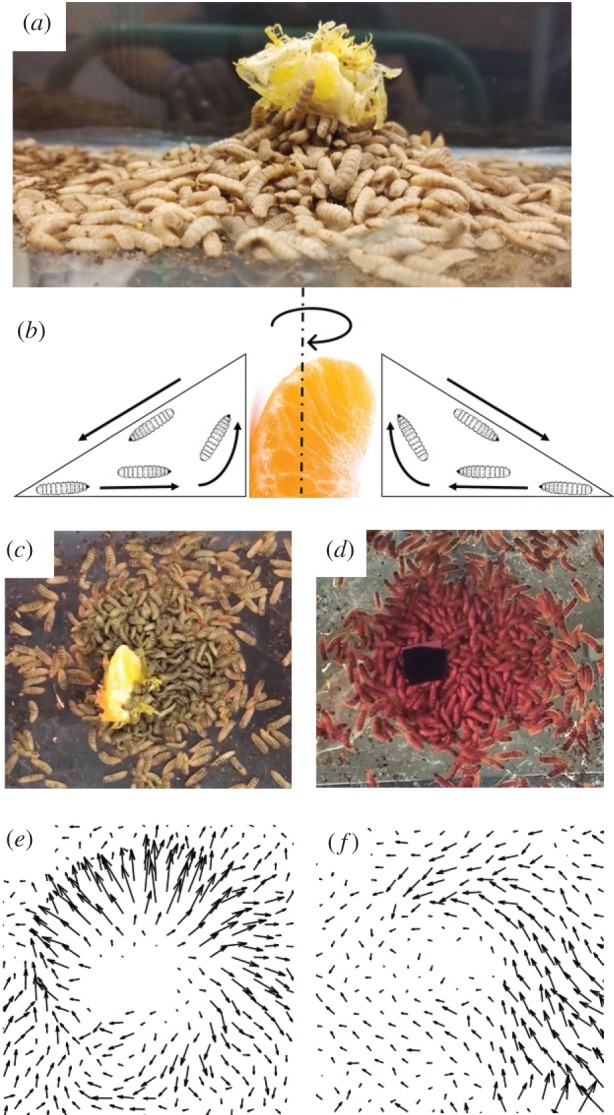
(a) Side view of larvae eating an orange slice by building a flowing fountain of larvae around the food. (b) Schematic of larva motion around an orange slice. (c,d) The region of flowing larvae, seen from above (c) and below (d). (e,f) Velocity fields associated with the views in (c,d). They are calculated using PIV and averaged over 2000 s. The centre is not analysed as it contains the orange slice. (Online version in colour.)

Filming from the top and bottom yields the views in figure 6c,d and the electronic supplementary material, videos S4 and S5, respectively. The naked eye sees that larvae move randomly, especially in the top view, but PIV can detect a coherent flow direction. In the top view in figure 6e, larvae form a radial outflow. In the bottom view in figure 6f, the larvae form a combination of a vortex and an inflow. The vectors are averaged over 2000 s, and their length indicates their relative magnitudes. The average velocities on the top and bottom layers are comparable in magnitude, of the order of 0.1 mm s⁻¹ or 0.007 body lengths per second, but much of this is part of the vorticity around the orange slice. Moreover, this speed is 20 times slower than the unimpeded speed of a single larva in a petri dish, 2 mm s⁻¹. The divergence and vorticity on the top and bottom layer are comparable in magnitude as well. The vorticity of the larvae on the bottom layer is negative of that from the top, as it is filmed from below and the axis is reversed; the entire aggregation of larvae therefore spins in the clockwise direction, from the top view.

Based on the top and bottom views, we surmise that physical picture is a fountain of larvae that are pumped inward and upward, as shown in the schematic in figure 6b. Larvae flow in from the bottom and flow out only on the top layer while the entire mixing region spins clockwise. In other words, net motion only occurs on the boundaries, the free surface and the substrate beneath the larvae. The details of the calculated velocity and other parameters for the top and bottom layers are shown in electronic supplementary material, table S2.

Snapshots from experiments using 500 to 10 000 larvae are shown in figure 3a–e on the left. Larvae primarily gather around the orange and in the corners of the container. Watching the videos with a naked eye shows that a well-defined mixing region is present. Vectors are calculated using PIV and averaged over a duration of 1500 s, starting at 500 s to ensure the mixing region is close to steady state. The average speed of larvae outside the mixing region and away from the corners is 0.05 ± 0.006 mm s⁻¹, calculated for the 10 000 larvae experiment. Using the minimum velocity threshold of 0.125 mm s⁻¹, we define the mixing regimes precisely using PIV, shown by the regions highlighted in red surrounded by a dashed border in the right column of figure 3a–e. The mixing region is not perfectly round and can be asymmetric, as shown for 1000 larvae in figure 3b. Higher numbers of larvae result in larger mixing regions, as can be seen by comparing the mixing regions for 500 and 10 000 larvae. Larvae also form outflows in the corners of the container similar to the outflow from the orange.

The relationship between the flow rate and group size is shown in figure 3f. We estimate the flow rate by assuming that the inflow or outflow occurs over a layer depth of one larva height (3.2 mm), and using equation (2.1). The flow rate increases linearly with number of larvae for 1000 and more larvae, as in equation (2.2): Q = 0.0075N + 64, R² = 0.60. This relationship will be used in our mathematical model where we estimate the feeding rate.

4.3. Eating rate as a function of group size

We feed orange slice pieces to groups of larvae ranging from 10 larvae to 58 000 larvae, spanning four orders of magnitude in size. Figure 4a shows an experiment with a simultaneous test of 1, 10, 100, 200 and 500 individuals. In the containers with 500 larvae, the orange slice is not visible because it is buried by larvae after 10 min of the experiment. In the containers with a single larva, the larva lays hidden under the orange slice without eating, and so that data point is not used.

As shown in electronic supplementary material, video S6, larvae rotate the orange slice as they consume it, but this rotation is bounded by the walls of the container. Figure 4b shows the relation between number of larvae N and their eating rate dM/dt. By plotting linear best fits to the small (N ≤ 500) and large (N ≥ 1000) numbers of larvae, we find they intersect at N₀ = 1300 larvae.

We use the properties of the orange slice, individual larvae and larva flow rates to model the eating rates of these larvae in three regimes, as in equation (3.8). Based on the surface area limit in equation (3.3), if a larva’s head is w = 4.3 mm wide by h = 3.2 mm tall, then the maximum number of larvae that can eat an orange with a surface area S = 4067 mm² at one time is N_max ∼ 337 larvae. This prediction for N_max is 1000 larvae below the experimentally found N₀. This is in part due to the calculation for N₀ not accounting for mixing of larvae, which allows more larvae to access food. Additionally, the experiments at higher numbers of larvae were done at higher temperatures, yielding higher eating rates (rather than increasing the number of larvae that can fit around food). Finally, there is a lot of scatter in the data at higher numbers of larvae, which may contribute to the discrepancy in N₀.

The average eating rate of one larva eating an orange is η ∼ 0.03 ± 0.02 g h⁻¹ (based on experiments with 10 larvae). Using our data on individual larva eating behaviour from single larva experiments and values for Q from the PIV experiments, we can calculate the threshold when the larvae mixing does not yield any additional eating, N′ ∼ 2850 larvae (equation (3.7)). The eating rates of larvae are calculated using our mathematical model given in equation (3.8). These predictions are depicted as dashed lines in figure 4b, which show close matching to experimental trends. Thus, the ‘fountain’ that larvae form around food increases their eating rates to a theoretical maximum, reached when there are N′ larvae in the container. The eating rate model is an underestimate of the actual eating rates with many larvae, likely due to the higher temperatures that experiments with large numbers of larvae were performed at.

Larvae can consume oranges very rapidly. If a larva weighing 0.1 g eats an orange slice at a rate of η ∼ 0.03 g h⁻¹, it will eat 6.5 times its body weight per day. This is of the same order of magnitude as the approximately 2 body weights per day they eat in chicken feed [2,3]. Oranges, which contain more liquid than chicken feed, can be consumed by larvae more quickly.

5. Discussion

When larvae are raised in industry, their food is blended and then mixed with the larvae aggregation to avoid the surface area limit and allow most larvae to eat to their maximum capacity. However, food pieces cannot be perfectly distributed between all larvae. Reducing the number of larvae in a bin and increasing the surface area of food pieces can help increase how quickly larvae eat food, leaving less to rot because larvae cannot access it.

The ‘fountain of larvae’ may not be possible for other animal species. Larvae crawl on top of one another to access food, while cattle and other land animals do not. Fish in schools avoid touching each other, while larvae touch one another constantly, and in fact do not like to be isolated. The feeding behaviour of other animals is affected by their social hierarchy [6,7], while larvae do not have complex social dynamics. Thus, fly larvae may be unique among scavengers in their group feeding abilities.

6. Conclusion

In this study, we investigate how groups of black soldier fly larvae feed. The number of larvae that can feed is intrinsically limited by the surface area of food, around which only limited numbers of larvae can fit. Moreover, larvae that are eating take frequent breaks, blocking others from accessing the food. Groups of larvae overcome these two problems by generating fountains around food, where new larvae crawl in from the bottom and are ‘pumped’ out of the top. We present a mathematical model that predicts the rate of eating as a function of group size, taking into account the pumping action.

Data accessibility

Data on eating rates, larva eating timing and results from PIV calculations are provided in the electronic supplementary material: Data_supplementary_FINAL.xlsx.

Authors' contributions

O.S. contributed to data collection and analysis, participated in the design of the study and drafted the manuscript. M.H. contributed to the PIV video recording and analysis. C.J. collected and analysed eating rate data. D.H. conceived, designed and coordinated the study and helped draft the manuscript. All authors gave final approval for publication.

Competing interests

We declare we have no competing interests.

Funding

This project has been supported with a commercialization grant from the Georgia Research Alliance, with NSF career award (PHY-1255127), by Grubbly Farms, by the Summer Undergraduate Research in Engineering/Sciences (SURE) programme and by the US Army Research Laboratory and the US Army Research Office Mechanical Sciences Division, Complex Dynamics and Systems Program, under contract no. W911NF-12-R-001.

References

- 1.Gustavsson J, Cederberg C, Sonesson U, Van Otterdijk R, Meybeck A. 2011. Global food losses and food waste: extent causes and prevention. Rome, Italy: Food and Agriculture Organization (FAO) of the United Nations. [Google Scholar]
- 2.Diener S, Zurbrugg C, Tockner K. 2009. Conversion of organic material by black soldier fly larvae: establishing optimal feeding rates. Waste Manag. Res. 27, 603–610. ( 10.1177/0734242X09103838) [DOI] [PubMed] [Google Scholar]
- 3.Makkar HP, Tran G, Heuzé V, Ankers P. 2014. State-of-the-art on use of insects as animal feed. Anim. Feed Sci. Technol. 197, 1–33. ( 10.1016/j.anifeedsci.2014.07.008) [DOI] [Google Scholar]
- 4.Sumpter DJ. 2006. The principles of collective animal behaviour. Phil. Trans. R. Soc. B 361, 5–22. ( 10.1098/rstb.2005.1733) [DOI] [PMC free article] [PubMed] [Google Scholar]
- 5.Hefti E, Trechsel U, Rfenacht H, Fleisch H. 1980. Use of dermestid beetles for cleaning bones. Calcif. Tissue Int. 31, 45–47. ( 10.1007/BF02407166) [DOI] [PubMed] [Google Scholar]
- 6.Nielsen BL, Lawrence AB, Whittemore CT. 1995. Effect of group size on feeding behaviour, social behaviour, and performance of growing pigs using single-space feeders. Livest. Prod. Sci. 44, 73–85. ( 10.1016/0301-6226(95)00060-X) [DOI] [Google Scholar]
- 7.Grant R, Albright J. 2001. Effect of animal grouping on feeding behavior and intake of dairy cattle. J. Dairy Sci. 84, E156–E163. ( 10.3168/jds.S0022-0302(01)70210-X) [DOI] [Google Scholar]
- 8.Evangelista DJ, Ray DD, Raja SK, Hedrick TL. 2017. Three-dimensional trajectories and network analyses of group behaviour within chimney swift flocks during approaches to the roost. Proc. R. Soc. B 284, 20162602 ( 10.1098/rspb.2016.2602) [DOI] [PMC free article] [PubMed] [Google Scholar]
- 9.Attanasi A. et al. 2014. Information transfer and behavioural inertia in starling flocks. Nat. Phys. 10, 691–696. ( 10.1038/nphys3035) [DOI] [PMC free article] [PubMed] [Google Scholar]
- 10.Dunkel J, Heidenreich S, Drescher K, Wensink HH, Bär M, Goldstein RE. 2013. Fluid dynamics of bacterial turbulence. Phys. Rev. Lett. 110, 228102 ( 10.1103/PhysRevLett.110.228102) [DOI] [PubMed] [Google Scholar]
- 11.Sanchez T, Chen DT, DeCamp SJ, Heymann M, Dogic Z. 2012. Spontaneous motion in hierarchically assembled active matter. Nature 491, 431–434. ( 10.1126/science.1093010) [DOI] [PMC free article] [PubMed] [Google Scholar]
- 12.Donev A, Cisse I, Sachs D, Variano EA, Stillinger FH, Connelly R, Torquato S, Chaikin PM. 2004. Improving the density of jammed disordered packings using ellipsoids. Science 303, 990–993. ( 10.1080/09500830500080763) [DOI] [PubMed] [Google Scholar]
- 13.Depickère S, Fresneau D, Deneubourg JL. 2004. The influence of red light on the aggregation of two castes of the ant, Lasius niger. J. Insect Physiol. 50, 629–635. ( 10.1016/j.jinsphys.2004.04.009) [DOI] [PubMed] [Google Scholar]
- 14.Thielicke W, Stamhuis EJ. 2014. PIVlab—towards user-friendly, affordable and accurate digital particle image velocimetry in MATLAB. J. Open Res. Softw. 2, 30 ( 10.5334/jors.bl) [DOI] [Google Scholar]
- 15.Thielicke W. 2014. The flapping flight of birds: analysis and application. PhD thesis, Rijksuniversiteit Groningen.
- 16.Delaney G, Weaire D, Hutzler S, Murphy S. 2005. Random packing of elliptical disks. Philos. Mag. Lett. 85, 89–96. ( 10.1080/09500830500080763) [DOI] [Google Scholar]
- 17.Kim WT, Bae SW, Park HC, Park KH, Lee SB, Choi YC, Han SM, Koh Y-H. 2010. The larval age and mouth morphology of the black soldier fly, Hermetia illucens (Diptera: Stratiomyidae). Int. J. Ind. Entomol. 21, 185–187. [Google Scholar]
Associated Data
This section collects any data citations, data availability statements, or supplementary materials included in this article.
Supplementary Materials
Data Availability Statement