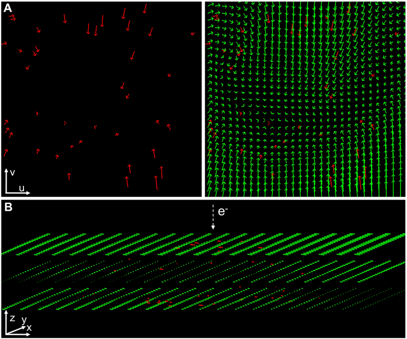
Figure 2. Estimation of the sample motion at the image plane in 3D by residual interpolation.

(A) An illustrative, simplified 2D case of residual interpolation. Left: residuals at scattered, discrete fiducial positions in a thin sample are presented with red arrows. The initial point of the arrows represents the expected fiducial position according to the standard projection model (i.e. $p_j^i=M^i{r}_j+d^i$) whereas the terminal point represents the experimental position (i.e. $q_j^i$). Right: Sample motion (green vectors) estimated by applying scattered data interpolation over the residuals in (a) (red vectors). For illustrative purposes, the residuals and their interpolated values are shown at the image plane (axes u, v of the image coordinate system; see Fig. 1). (B) Residual interpolation in 3D. Residuals at scattered, discrete 3D fiducial coordinates (r_j) obtained for the untilted image from a thick sample are presented with red lines in the 3D sample coordinate system (axes x,y,z, see Fig. 1). These residuals $\left(q_j^i-p_j^i\right)$ represent shifts perpendicular to the electron beam direction, as observed at the image plane (Fig. 1). After scattered data interpolation, the sample motion is estimated for every point in the tomogram (green vectors; these discrete vectors are represented in a grid and, for clarity, only three Z-planes of this grid are presented). All vectors shown in the figure were scaled 10×.