Figure - PMC

Skip to main content

An official website of the United States government

Here's how you know

Here's how you know

Official websites use .gov
A .gov website belongs to an official government organization in the United States.

Secure .gov websites use HTTPS
A lock ( ) or https:// means you've safely connected to the .gov website. Share sensitive information only on official, secure websites.

View full-text article in PMC

. 2019 Mar 18;9:4790. doi: 10.1038/s41598-019-41250-w

Search in PMC
Search in PubMed
View in NLM Catalog
Add to search

© The Author(s) 2019

Open Access This article is licensed under a Creative Commons Attribution 4.0 International License, which permits use, sharing, adaptation, distribution and reproduction in any medium or format, as long as you give appropriate credit to the original author(s) and the source, provide a link to the Creative Commons license, and indicate if changes were made. The images or other third party material in this article are included in the article’s Creative Commons license, unless indicated otherwise in a credit line to the material. If material is not included in the article’s Creative Commons license and your intended use is not permitted by statutory regulation or exceeds the permitted use, you will need to obtain permission directly from the copyright holder. To view a copy of this license, visit http://creativecommons.org/licenses/by/4.0/.

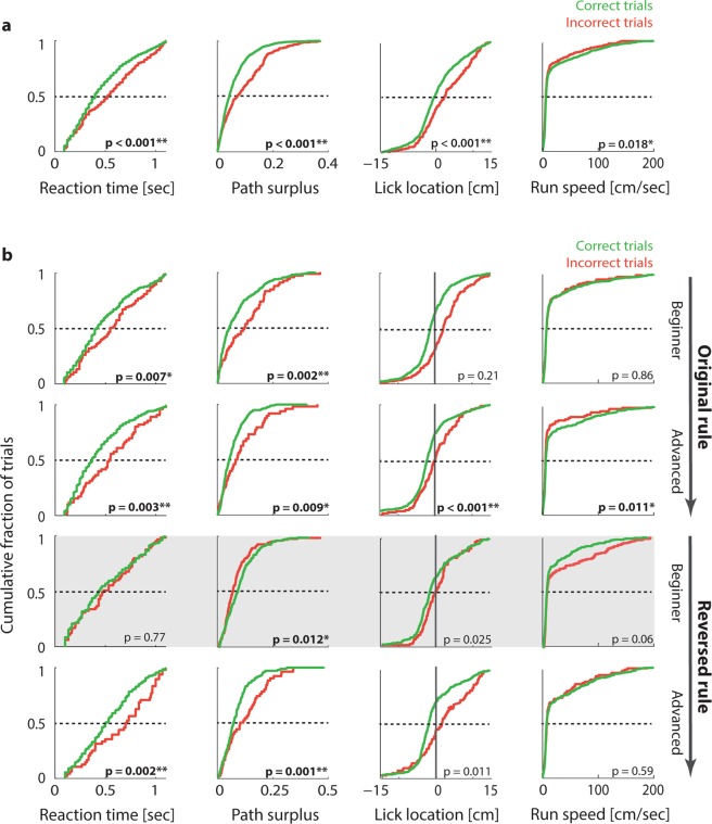
PMC Copyright notice

After rule acquisition mice are able to predict errors. (a) Differences in reaction time, path surplus, running speed and lick location for correct versus incorrect trials, pooled across five animals in the original task. Left panel: Cumulative distribution function (CDF) of reaction times, pooled across animals for all trials of the original task. Green: Correct trials. Red: Incorrect trials. Insets: P-values resulting from a Kolmogorov-Smirnov test of the distribution differences between correct and incorrect trials (*p < 0.05; **p < 0.01 after correction for multiple comparisons; see Methods). (b) Differences in reaction time, path surplus, running speed and lick location for correct versus incorrect trials, at different stages of rule acquisition. Top row: Cumulative distribution function (CDF) of reaction times (left), path surplus (centre left), lick positions (centre right) and running speed (right), for the first 30% of trials of ΔOri = 30° or easier, beginning at training stage 5, pooled across all animals. Green: Correct trials. Red: Incorrect trials. Insets: p-values resulting from a Kolmogorov-Smirnov test of the distribution differences between correct and incorrect trials (*p < 0.05; **p < 0.01 after correction for multiple comparisons; see Methods). Second row: Same for the last 30% of trials of ΔOri = 30° or easier in the original task. Third row: Same for the first 30% of trials of ΔOri = 30° or easier after the first rule reversal. Grey shade in background highlights that this is the time point when distribution differences are transiently diminished (reaction time, path surplus and licking position) and/or reversed (path surplus and running speed). Bottom row: Same for the final 30% of trials of ΔOri = 30° or easier after the first rule reversal.