Estimation of Random Coefficient Multilevel Models in the Context of Small Numbers of Level 2 Clusters

Abstract

Multilevel data are a reality for many disciplines. Currently, although multiple options exist for the treatment of multilevel data, most disciplines strictly adhere to one method for multilevel data regardless of the specific research design circumstances. The purpose of this Monte Carlo simulation study is to compare several methods for the treatment of multilevel data specifically when there is random coefficient variation in small samples. The methods being compared are fixed effects modeling (the industry standard in business and managerial sciences), multilevel modeling using restricted maximum likelihood (REML) estimation (the industry standard in the social and behavioral sciences), multilevel modeling using the Kenward–Rogers correction, and Bayesian estimation using Markov Chain Monte Carlo. Results indicate that multilevel modeling does have an advantage over fixed effects modeling when Level 2 slope parameter variance exists. Bayesian estimation of multilevel effects can be advantageous over traditional multilevel modeling using REML, but only when prior probabilities are correctly specified. Results are presented in terms of Type I error, power, parameter estimation bias, empirical parameter estimate standard error, and parameter 95% coverage rates, and recommendations are presented.

Introduction

Multilevel data arise when lower level sampling units (e.g., students) are nested within higher level sampling units (e.g., schools). This multilevel structure can occur at more than two levels, for example, when students are nested in classrooms, which are in turn nested within schools. Such structure needs to be accounted for in data analysis, otherwise model parameters, particularly standard errors, will be biased (Snijders & Bosker, 2012). Multilevel data is a reality for many different areas of research, including the social, behavioral, educational, medical, and managerial sciences. Given the prevalence of this issue across disciplines, it is interesting that there appear to be differences in terms of how researchers from different fields choose to analyze multilevel data. For example, researchers in the social, educational, and behavioral sciences frequently use a family of methods called multilevel modeling (MLM) for such analyses, whereas those working in business and management research often use fixed effects models (FEM) for analysis of multilevel data (McNeish & Stapleton, 2016). Recent work has discussed the theoretical differences between MLM and FEM, and their application to multilevel data structures (Chaplin, 2003; Galbraith, Daniel, & Vissel, 2010; Huang, 2016; McNeish, Stapleton, & Silverman, 2017; Setodji & Shwartz, 2013).

An issue that has not been completely resolved with respect to multilevel data modeling involves the best approach for dealing with situations where higher level sample sizes are relatively small. In studies that have addressed this issue (e.g., McNeish & Stapleton, 2016), two alternative approaches for MLM have been described, a variant for MLM allowing for smaller Level 2 cluster sizes known as the Kenward–Roger (KR) correction and Bayesian estimation using a Markov Chain Monte Carlo (MCMC) approach.

The purpose of the present study was to compare standard MLM estimation with several alternative estimation approaches, including FEM, MLM with the KR correction, and MCMC, when there is random slope variation, particularly when samples are small. Although FEM is not subject to the assumption of endogeneity and thus does not need all predictors present to be unbiased, it is unclear how FEM will compare with more complex models when random slope variation is indeed present. MLM would generally be the method of choice as it allows for direct modeling of random slope variation; however, it is unknown how it will compare to FEM or other complex methods when higher level samples are small. Following are descriptions of each method included in the present simulation study.

Multilevel Modeling (Using REML Estimation)

In the social, educational, and behavioral sciences, when multilevel/nested data are encountered, the standard analysis involves fitting MLMs using restricted maximum likelihood (REML) estimation. As described by Raudenbush and Bryk (2002), this approach accounts for the multilevel structure of data by allowing for predictors at all levels of analysis to be used. In order to accomplish this, prediction equations are created for each level of the nested structure. The Level 1 equation involves simple prediction of the outcome from Level 1 (e.g., student) characteristics much like the prediction equation of a traditional regression model. This relationship is demonstrated in Equation (1), where Y_ij is the outcome for individual i in group j, β₀₀ is the intercept of the Level 1 equation, β₁₀ is a slope for a Level 1 predictor variable, and r_ij is the Level 1 error term.

$$Y_{\mathrm{ij}}={\beta }_{00}+{\beta }_{10}\left(X_{\mathrm{ij}}\right)+r_{\mathrm{ij}}$$

In order to account for variance from higher levels of analysis, Level 2 (and higher) prediction equations can be used to obtain estimates of the intercept and slope coefficients from the Level 1 model. As can be seen in Equations (2) and (3), γ₀₀ is the intercept for the prediction equation for β₀₀ (which in most cases is interpreted as the grand mean), γ₁₀ and γ₀₁ are slope coefficients for the prediction of the Level 1 coefficients, and u_0j and u_1j are unique or random effects associated with the Level 1 intercept and slope, respectively.

$${\beta }_{00}={\gamma }_{00}+{\gamma }_{01}\left(Z\right)+u_{\mathrm{oj}}$$

$${\beta }_{10}={\gamma }_{10}+{\gamma }_{11}\left(Z\right)+u_{1j}$$

Considering Equations (2) and (3), it is evident that MLM provides a very flexible framework for understanding nested effects by allowing for predictors at multiple levels of analysis, accounting for multiple levels of data structure (sample size permitting), and accommodating model customization such as cross-level interactions, variation in coefficients (β₀₀, β₁₀) at higher data levels, or use with categorical outcomes. MLM generally requires relatively larger sample sizes (Hox, 2010) and is subject to reasonably strict assumptions about the sample and data distributions (Raudenbush & Bryk, 2002). Given these potential limitations with respect to sample size, it seems important to consider other possible options for the analysis of multilevel data.

The Kenward–Roger Correction

The KR correction is described in detail in Kenward and Roger (2009), and thus the interested reader is referred there for a more in-depth discussion of the calculations. The purpose of the correction is twofold, namely, to address problems of negative bias in the standard errors of Level 1 model parameter estimates and to correctly approximate the denominator degrees of freedom in the hypothesis tests used to assess statistical significance for these estimates. These issues are not typically problematic in the context of sufficiently large Level 2 sample sizes, because of the asymptotic properties associated with the test statistics, and the sufficient amount of information in the sample necessary for accurate estimation (Kenward & Roger, 2009). However, with a small number of Level 2 units these desirable properties are no longer available. Kenward and Roger proposed their correction to the coefficient standard errors, using a modified Taylor Series expansion first described by Kackar and Harville (1984). In addition, they also developed a technique to approximate the denominator degrees of freedom for the hypothesis tests that is based on the commonly used Satterthwaite approach (Satterthwaite, 1946). Taken together, these methods have been shown to yield more accurate hypothesis testing results in the context of small number of units at Level 2 (e.g., McNeish & Stapleton, 2016).

Fixed Effects Models

While MLM has historically been the gold standard for analysis of multilevel data in the social, educational, and behavioral sciences, it is not as frequently used in the fields of business and econometrics. When researchers in these fields encounter multilevel data, they are quite likely to use FEM. Allison (2009) noted that FEMs provide the data analyst with a simpler model to account for the influence of higher levels in the data structure by including dummy variables for each Level 2 unit as fixed effects in a regression model. For example, if a researcher were dealing with a dataset containing students nested within schools, in the context of FEM the variance associated with schools would be accounted for by assigning a dummy variable to each of the schools. Regarding the dummy coding of Level 2 units, dummy variables can either be created as absolute, meaning all Level 2 units have a dummy variable and the intercept is omitted, or reference, meaning one Level 2 unit is left out and the intercept is retained. Using an absolute coding scheme, the FEM model can be represented as shown in Equation (4) where b_n are regression coefficients for Level 1 model covariates (X) and c_k are regression coefficients for Level 2–unit dummy variables (α).

$$Y_{\mathrm{ij}}=\sum b_n\left(X\right)+\sum c_k\left(\alpha \right)+r$$

Regardless of dummy coding scheme, when the FEM is used, the focus is on the interpretation of the relevant Level 1 covariates. The dummy variable context effects are generally not interpreted and are included in order to account for Level 2 variance. Representing Level 2 context effects in this manner allows for such variance to be accounted for, thereby yielding unbiased estimates of standard errors for Level 1 parameter estimates (Allison, 2009). FEM does not, however, allow for the specific effects of Level 2 covariates to be examined.

Markov Chain Monte Carlo

Bayesian estimation using the MCMC estimator has been suggested as being advantageous for small sample cases, including in the context of multilevel data (Gelman, 2006). Given space limitations, and the plethora of literature describing MCMC estimation, we will not delve deeply into this topic here. Readers who would like to learn more about the details of Bayesian estimation using MCMC are referred to Kaplan (2014) and Congdon (2003) for a general treatment of the topic. With regard to MLM specifically, Browne and Draper (2006) provide discussion of the topic as well. Very briefly, the use of MCMC estimation requires that the researcher select a prior distribution for each of the model parameters, which are themselves conceptualized as distributions rather than as single values as in the frequentist analysis paradigm that underlies REML estimation. The MCMC algorithm combines this prior information with information taken from the data in order to estimate the distribution of the parameter, which is referred to as the posterior distribution. When samples are small, the selection of these priors is very important because they will have a relatively large impact on the nature of the posterior distributions (Kaplan, 2014). In other words, in the absence of much observed data, the posterior will rely more heavily on the prior distribution. McNeish and Stapleton (2016) addressed this issue by comparing MCMC using several different prior distributions and found that the inverse gamma and the half-Cauchy prior distributions for the Level 2 variances both performed best among the options that they examined. Given these results, the inverse gamma distribution was used as the prior for the variance components of the Level 1 parameters in the current study.

Prior Research on Small Samples and Multilevel Analysis

The majority of research comparing different types of multilevel analysis has focused on MLM compared with FEM as these are the “industry standards.” Much of this discussion has revolved around a comparison of the assumptions for these methods. Due to its more complex structure, MLM has more strict assumptions than FEM. One major point of difference between the two modeling paradigms is that MLM assumes all relevant predictors and all relevant random effects are included in the model, and that all covariance structures (i.e., the covariance structure of the within-cluster residuals and the covariance structure of the random effects) are properly specified. Thus, in order for MLM to produce unbiased estimates, the model needs to be properly specified both in terms of variables chosen and model structure. Any omitted Level 2 variables can bias the Level 1 slope estimates, a problem that does not occur in FEM (Chaplin, 2003). The inclusion of Level 2 dummy variables in FEM already ensures that all Level 2 variance is accounted for without requiring specific modeling (Allison, 2009). This relates closely to the assumption of MLM known as endogeneity. The assumption of endogeneity requires there to be a lack of correlation between within-cluster residuals and both the random effects and the predictor variables at any level. The assumption of endogeneity is often violated when necessary predictor variables are omitted (Raudenbush & Bryk, 2002). Thus, FEM is often suggested as an alternative when the assumption of endogeneity is questionable.

Within the last decade, there has been an increased focus in empirical research on the estimation for multilevel data with small samples at Levels 1 and 2, and extending beyond FEM and traditional MLM. The goal of several of these simulation studies has been to identify estimators and adjustments to estimators that yield efficient and unbiased parameter estimates with a small number of clusters at Level 2. Among other findings, several of these studies have found that when the standard REML estimator is employed it is necessary to have at least 30 Level 2 units in order to obtain unbiased estimates with standard errors that are in control (e.g., Bell, Morgan, Schoeneberger, Kromrey, & Ferron, 2014; Maas & Hox, 2005). Kenward and Roger (2009) demonstrated that their correction for small sample MLM estimation could lower the required number of Level 2 clusters to as few as 10 in some cases when the goal was to accurately estimate the random intercept and error variance components. Bayesian estimation based on the MCMC algorithm has also been suggested for use with small sample multilevel data and has been shown to be quite effective for estimating the random intercept and error variances, if correct informative priors are selected (Browne & Draper, 2006; Ferron, Bell, Hess, Rendina-Gobioff, & Hibbard, 2009; Gelman, 2006; Hox, van de Schoot, & Matthijsse, 2012).

One of the limitations of the work cited above is that these various methods for estimating multilevel models were not compared directly with one another in the context of a small number of Level 2 units. Recently, McNeish and Stapleton (2016) addressed this gap in the literature by conducting an extensive Monte Carlo simulation study in which they compared these approaches with small Level 2 samples. This study was the first to examine the performance of several methods together, including MLM using REML, MLM using REML with the KR, MCMC using three different prior distributions for the variance components, as well as generalized estimating equations, and FEMs. The outcomes of interest were parameter estimate relative bias, coverage, and power rates for the Level 1 regression coefficient, the Level 1 residual variance estimate, and the Level 2 intercept variance estimate. The results of the McNeish and Stapleton (2016) study revealed that multiple approaches can be used to obtain accurate estimates of the parameters in question, with reasonable coverage and power rates. For example, with regard to the Level 1 regression parameter estimate, FEM was found to yield estimates with low levels of bias, and with higher power for identifying non-0 values in the population than was true for the other methods. Bias in the regression coefficients for KR was also low across conditions. With regard to the variance component estimates, REML performed poorly for fewer than 10 clusters, with lower than nominal coverage rates for the parameter estimate. However, KR was able to address this problem for the most part, with the exception of the 4 clusters condition, for which coverage was nearly as low as for the uncorrected REML approach. Among the Bayesian estimation techniques, MCMC using the inverse gamma(0.01, 0.01) prior distribution, and MCMC with a Half-Cauchy(0,4) prior for the model variance components yielded low parameter estimation bias, and high coverage and power rates. The final recommendations from McNeish and Stapleton were to consider the use of MCMC with the inverse gamma prior, and FEM, if the primary goal of the analysis is to estimate a Level 1 regression relationship and not the variance components.

Study Goals

As noted above, the purpose of the current study is to build on earlier research examining the impact of sample size, at both Levels 1 and 2, on the performance of several estimators for multilevel models in the context of random coefficient effects. The methods that were used in this study include FEM, REML, KR, MCMC with noninformative inverse gamma priors for the variance components, and MCMC with informative inverse gamma priors. Prior work, which was reviewed above, has found that the number of Level 2 units (clusters), as well as the total sample size (clusters × sample per cluster) will have an impact on the estimation of the random intercept and Level 1 residual components in MLMs. Specifically, as noted above, the FEM and KR approaches were found to be particularly promising for use when there are a small number of clusters at Level 2 and the interest is in obtaining accurate estimates and coverage rates for the Level 1 regression coefficients and variance component values using KR (McNeish & Stapleton, 2016). The current study extends this line of research by comparing the most promising estimators identified in the earlier research, for models where the coefficient relating a Level 1 predictor and the outcome variable has a random component, that is, a random coefficients model. Based on the earlier studies cited above, several hypotheses regarding the current study are suggested.

• Hypothesis 1: With regard to estimating the fixed effects portion of the Level 1 coefficient, it is anticipated that each of the methods should provide unbiased estimates across sample sizes. This is a result that has been found in prior work (e.g., McNeish & Stapleton, 2016). It is not known, however, what impact the Level 2 random component of the coefficient might have on estimation of the Level 1 fixed portion.

• Hypothesis 2: Based on earlier research, it is hypothesized that FEM will yield the highest power rates for the Level 1 regression coefficient and that all the methods will control the Type I error rate for this test. It is important to note, however, that prior simulation studies included only a fixed effects component to the coefficient, so that little is known about what impact a random coefficient might have on these estimators.

• Hypothesis 3: Prior research has indicated that estimation of the Level 2 intercept variance component is affected by the number of Level 2 clusters, and the same is expected to be the case for the Level 2 coefficient variance component in the current study. Specifically, it is anticipated that the KR coverage rates for the random coefficient parameter estimate will be superior to those for REML, and that those for the model based on informative MCMC priors will be the best of all.

Method

A Monte Carlo simulation study was used to address the research goals outlined above. A total of 1,000 replications were generated for each combination of the manipulated conditions, which are described here. All the manipulated study conditions were completely crossed with one another, with the exception of the FEM estimator, as is discussed below. Data were generated using Mplus version 7.11 (Muthén & Muthén, 1998-2017), and data analyses were conducted using SAS version 9.3 (SAS Institute, 2015). The intraclass correlation was set at 0.2 across manipulated study conditions. This value has been used in prior research (e.g., French & Finch, 2013; McNeish & Stapleton, 2016) and represents a moderate level of correlation within the Level 2 clusters. A number of conditions were manipulated in this study and were selected in order to build on prior research in this area as well as to reflect conditions that are seen in practice.

Data Generating Models

Two data generating models were used in the current study. Model 1 included only a single Level 1 predictor (which served as the target of the simulation study), with both a random intercept and random slope term, and took the form:

$$y_{\mathrm{ij}}={\gamma }_{00}+{\gamma }_{10}{x}_{1\mathrm{ij}}+U_{0j}+U_{1j}{x}_{1\mathrm{ij}}+{\epsilon }_{\mathrm{ij}}$$

where $y_{\mathrm{ij}}$ is the dependent variable value for subject i in cluster j; simulated from the $N(0,1)$ distribution; ${\gamma }_{00}$ is the fixed intercept effect; set at 1 in simulations; ${\gamma }_{10}$ is the fixed coefficient effect for predictor x; manipulated as described below; $x_{1\mathrm{ij}}$ is the target predictor variable value for subject i in cluster j; simulated from the $N(0,1)$ distribution; $U_{0j}$ is the random intercept variance; simulated from the $N(0,1)$ distribution; $U_{1j}$ is the random coefficient variance for predictor x₁; manipulated as described below; and ${\epsilon }_{\mathrm{ij}}$ is the random residual variance; simulated from the $N(0,1)$ distribution.

Model 2 was simulated to include the target predictor from Model 1 as well as a second Level 1 predictor and a Level 2 predictor. The purpose of including Model 2 was to investigate the performance of the various estimators with more complex models, for which the burden of the small samples could potentially be greater. Model 2 took the following form:

$$y_{\mathrm{ij}}={\gamma }_{00}+{\gamma }_{10}{x}_{1\mathrm{ij}}+{\gamma }_{20}{x}_{2\mathrm{ij}}+{\gamma }_{01}{z}_{\mathrm{ij}}+U_{0j}+U_{1j}{x}_{1\mathrm{ij}}+{\epsilon }_{\mathrm{ij}}$$

where ${\gamma }_{20}$ is the fixed coefficient effect for Level 1 predictor $x_2$; set at 0.5 in all simulations; $x_{2\mathrm{ij}}$ is the value of second Level 1 variable; simulated from the $N(0,1)$ distribution; ${\gamma }_{01}$ is the coefficient for Level 2 predictor; set at 0.5 in all simulations; and $z_{\mathrm{ij}}$ is the value of Level 2 predictor; simulated from the $N(0,1)$ distribution.

Number of Clusters and Sample Size Per Cluster

The number of Level 2 units was set at 5, 10, 15, or 20, taking values in the range of those that have been used in previous research focusing on estimation of Level 2 intercept variance (e.g., Kenward & Roger, 2009; Maas & Hox, 2005; McNeish & Stapleton, 2016; Schoenberger, 2016). These values are also representative of a number of studies that take place in educational research contexts where researchers gather data from a relatively small number of schools or classrooms. The sample size per cluster (i.e., number of Level 1 units) was set at 10, 20, 30, and 40, again falling within the range of other research in the area of small sample MLM estimation. Thus, the total sample sizes ranged from 50 to 800.

Magnitude of the Level 1 Slope

The fixed effects portion of the target predictor coefficient was set at 0, 0.2, 0.4, 0.6, and 0.8. Given that the data were generated from a standard normal distribution, these values can be interpreted as representing no relationship between the predictor and the outcome variable (0), a small relationship (0.2), a moderate relationship (0.4 and 0.6), and a large relationship (0.8). In other words, a large relationship was operationalized as being 0.8 of a standard deviation of the dependent variable, and a small relationship was operationalized as being 0.2 of a standard deviation.

Magnitude of the Level 2 Slope Variance Component

The magnitudes of the Level 2 variance component for the Level 1 coefficient (i.e., random coefficient effect) were 0.25, 0.5, and 0.75. These values were selected so as to represent relatively low between-group variation in the relationship between the target predictor and the dependent variable (0.25), a moderate level of between-group variance (0.50), and a relatively large amount of between-group variance (0.75). These results are based on prior educational research in which random coefficient models have been employed (e.g., Escobar et al., 2013; Morgan & Sideridis, 2006 ; Timmermans, Kuyper, & van der Werf, 2015).

Estimation Methods

The estimation methods examined in this study were FEM, MLM using REML, MLM using REML with the KR correction, MCMC with noninformative inverse gamma(0.01, 0.01) priors for the Level 2 variance components, and MCMC with informative inverse gamma priors for the Level 2 variance components. For the informative gamma priors, values for the parameters (α and β) were selected so that the prior location value was equal to the parameter value, and the variance was 0.01. These were manipulated in the Mplus software using methods outlined in Asparouhov and Muthén (2010). The priors for the random intercept and Level 1 error were taken from the noninformative gamma(0.01, 0.01), and the noninformative prior for the fixed effect coefficient was taken from the normal (0, infinity) distribution. FEM, MCMC, REML, and KR were carried out using SAS version 9.3. The estimation methods included in this study were selected based on findings in prior studies, coupled with the focus of the current research on the estimation of the random coefficient parameter. Therefore, no GEE approaches were included in the study. McNeish and Stapleton (2016) found that GEE was relatively less effective for estimating the fixed effects parameters than were FEM, REML, or MCMC. In addition, GEE will not provide an estimate of the random coefficient variance, as will MCMC or REML. FEM will also not provide such an estimate; however, its superior performance in estimating the fixed portion of the coefficient, as reported in prior research, led us to include it in the current study. Finally, for Model 2, which included a Level 2 predictor, FEM was fit using only the Level 1 predictors, under the assumption that the Level 2 predictor effect would be captured in the cluster variable effect, as described by Allison (2009). When convergence was not obtained for a replication of a particular estimation method, then additional replications were run in the simulation until a total of 1,000 successful replications were obtained for each method across all combinations of study conditions.

Outcomes

As noted above, the goal of this study was to investigate the impact of small Level 2 sample sizes on the estimation of the fixed and particularly the Level 2 variance component of the regression coefficient relating a target variable to a continuous dependent variable (γ₁₀ and U_1j from Models 5 and 6, respectively). The outcomes of interest in this study included convergence rates, parameter estimation bias, empirical parameter estimate standard error, parameter 95% coverage rates, and Type I error/power rates for the Level 1 regression coefficient, and the Level 2 variance component estimate for the coefficient. The empirical standard error was calculated as the standard deviation of the parameter estimates across simulation replications. The nominal Type I error was set at 0.05 for both the coefficient and variance component estimates. In order to identify study factors that were related to each of the outcomes, analysis of variance (ANOVA) was used with the independent model terms being the main effects and interactions of the manipulated variables described above. For the Type I error and coverage rates, values were summarized across the 1,000 replications for each combination of study conditions, and then subjected to the ANOVA. In addition to tests of significance, the η² effect size was used to identify ANOVA model terms that accounted for at least 10% of the variance in each outcome variable. Thus, in order to warrant further investigation, a main effect or interaction had to be statistically significant (α= .05) and had to account for at least 10% of the variance in the outcome variable. The use of α= .05) is commonly used in simulation research (e.g., McNeish & Stapleton, 2016). An η² effect size criterion of 0.1 for identifying an important effect was selected both because it corresponds to the ANOVA model term accounting for 10% of the variance in the outcome variable, and because it falls within the moderate effect size range, as recommended by Cohen (1988).

Results

Convergence Rates

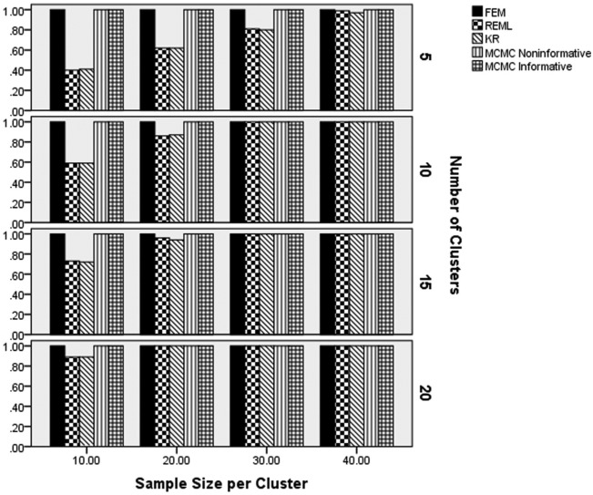
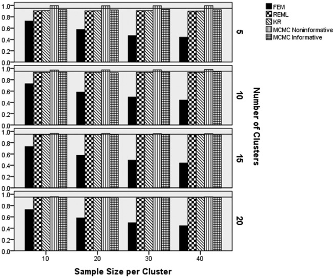
Convergence rates by method, sample size per cluster, and number of cluster appear in Figure 1. These results show that FEM and the two MCMC estimators had coverage rates at or near 1.00 across simulated conditions. Conversely, the REML and KR estimators had lower convergence rates for fewer Level 2 units, as well as for fewer Level 1 units. Convergence rates for these two approaches were lowest for the smallest total sample sizes (e.g., 5 Level 2 units and 10 individuals per units). When the sample size per cluster was 30 or 40, and the number of Level 2 units was 10 or more, the convergence rates for REML and KR were comparable to those for FEM, and the two MCMC methods.

Figure 1.

Convergence rates by estimation method, number of clusters, and sample size per cluster.

Note. FEM = fixed effects modeling; REML = multilevel modeling using restricted maximum likelihood estimation; KR = Kenward–Rogers correction for multilevel modeling; MCMC = Markov chain Monte Carlo with informative or noninformative priors.

Coefficient Parameter Estimate

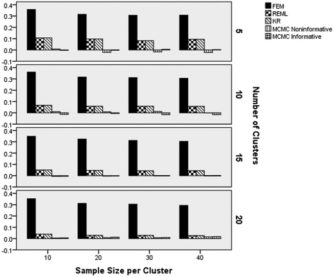
ANOVA results identified the interactions of estimation method by number of clusters by sample size ($F_{27,567}=12.76,p<.001,{\eta }^2=0.38$), and estimation method by slope population magnitude by slope random variance ($F_{18,567}=12.28,p<.001,{\eta }^2=0.28$) as the highest order statistically significant terms with respect to coefficient parameter estimation bias. All other terms were either not statistically significant, or were subsumed in one of these interactions. Figure 1 contains the slope parameter estimation bias by the number of clusters, sample size per cluster, and the estimation method. As evidenced by Figure 2, the FEM slope estimate displayed the highest levels of bias across sample size per cluster and number of clusters. This bias was lower for larger sample sizes per cluster, but always remained higher than that of any of the other methods. From Figure 2, it is also evident that the lowest parameter estimate bias was associated with the two MCMC estimators, whereas the parameter estimate bias of REML and KR were higher than those of MCMC. This was particularly evident with smaller numbers of clusters.

Figure 2.

Slope parameter estimation bias by estimation method, number of clusters, and sample size per cluster.

Note. FEM = fixed effects modeling; REML = multilevel modeling using restricted maximum likelihood estimation; KR = Kenward–Rogers correction for multilevel modeling; MCMC = Markov chain Monte Carlo with informative or noninformative priors.

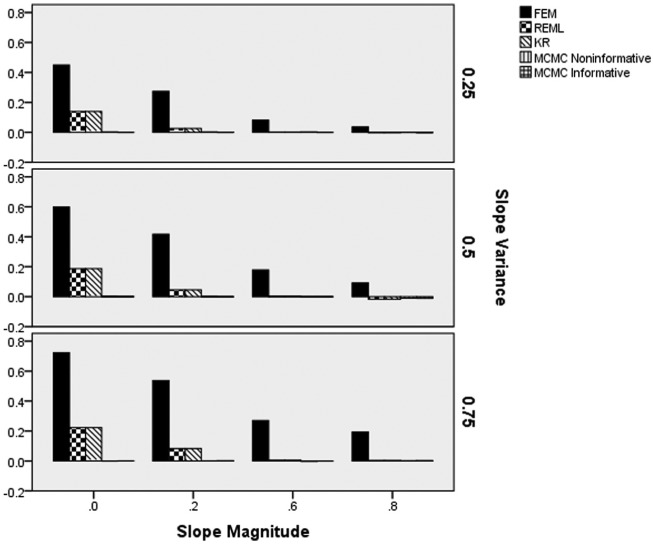
Figure 3 displays the slope parameter estimation bias by the slope variance, slope magnitude, and estimation method. It is clear from the figure that estimation bias for FEM, as well as REML and KR increases concomitantly with increased slope variance, for the lower magnitudes of the slope in the population. This increase in the slope estimation bias was more pronounced for the FEM approach, as compared with the REML and KR. In contrast to these three techniques, the estimation bias for the two MCMC techniques remained below that of the other methods, with values all less than 0.01. When the slope magnitude was 0.6 or 0.8, the bias of REML and KR was comparable to that of both MCMC approaches. However, for lower such magnitudes the MCMC methods both yielded lower estimation bias than any of the other methods.

Figure 3.

Slope parameter estimation bias by estimation method, slope magnitude, and population slope variance.

Note. FEM = fixed effects modeling; REML = multilevel modeling using restricted maximum likelihood estimation; KR = Kenward–Rogers correction for multilevel modeling; MCMC = Markov chain Monte Carlo with informative or noninformative priors.

Slope Estimate Standard Errors

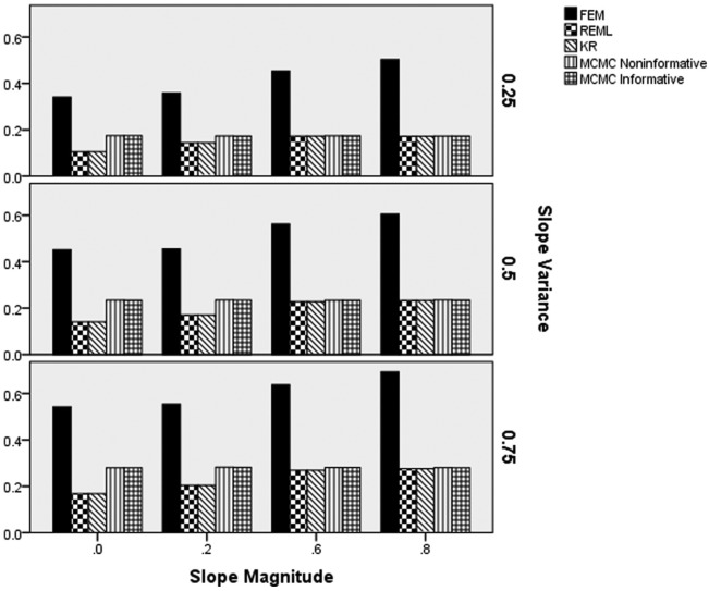
The results of the ANOVA indicated that the interaction of estimation method by population slope magnitude by population slope variance ($F_{18,567}=13.07,p<.001,{\eta }^2=0.29$), the interaction of estimation method by number of clusters ($F_{9,567}=32.63,p<.001,{\eta }^2=0.34$), and the interaction of estimation method by sample size ($F_{9,567}=20.20,p<.001,{\eta }^2=0.24$) were all statistically significantly related to the empirical standard error of the slope estimates. Figure 4 includes the empirical standard error values by estimation method, slope magnitude, and slope variance. Figure 4 clearly shows FEM to have the largest standard errors across all levels of the slope magnitude and slope variance. In addition, for all estimation methods, slope standard errors were larger for larger slope variances. Finally, REML and KR had the smallest standard errors when the slope magnitudes were 0 and 0.2, whereas their standard errors were comparable to those of the MCMC estimators for slope magnitudes of 0.6 and 0.8. This latter result is due to the fact that the standard errors of REML and KR increased in value for larger slope magnitudes, as opposed to the standard errors of MCMC declining. This increase in standard error value was approximately 0.08 in magnitude across slope variance magnitudes.

Figure 4.

Slope parameter empirical standard error by estimation method, slope magnitude, and slope variance.

Note. FEM = fixed effects modeling; REML = multilevel modeling using restricted maximum likelihood estimation; KR = Kenward–Rogers correction for multilevel modeling; MCMC = Markov chain Monte Carlo with informative or noninformative priors.

Table 1 includes the empirical standard errors by method, number of clusters, and sample size per cluster. As noted above, FEM had the largest standard errors of the methods studied here and varied little across conditions (between .50 and .55). For each of the other methods, the standard error declined with increases in the number of clusters and the sample size per cluster. In addition, REML and KR had the lowest standard errors (between .26 and .14), with the gap between these techniques and the two MCMC estimators narrowing with increases in the number of clusters and the sample size per cluster.

Table 1.

Empirical Standard Error by Estimation Method, Number of Clusters, and Sample Size per Cluster.

				MCMC
Number of clusters	FEM	REML	KR	Noninformative	Informative
5	.51	.26	.26	.33	.33
10	.51	.20	.20	.23	.23
15	.51	.16	.16	.19	.19
20	.51	.14	.14	.16	.16
				MCMC
Sample size per cluster	FEM	REML	KR	Noninformative	Informative
10	.55	.20	.20	.24	.24
20	.51	.19	.19	.23	.23
30	.50	.18	.18	.22	.22
40	.50	.19	.19	.22	.22

Note. FEM = fixed effects modeling; REML = multilevel modeling using restricted maximum likelihood estimation; KR = Kenward–Rogers correction for multilevel modeling; MCMC = Markov chain Monte Carlo with informative or noninformative priors.

Slope Parameter Estimate Coverage

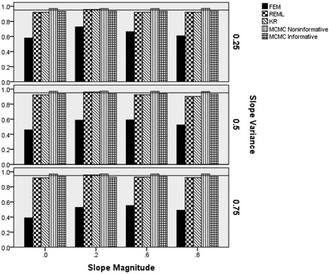
ANOVA identified that, as with the standard error estimate, the interaction of estimation method by the population slope magnitude by the population slope variance ($F_{24,567}=6.06,p<.001,{\eta }^2=0.16$) was statistically significantly related to the slope parameter coverage rate. In addition, the interaction of estimation method by number of clusters by sample size per cluster ($F_{36,756}=4.44,p<.001,{\eta }^2=0.18$) was also significantly related to the slope coverage rate. Figure 5 contains the coverage rates by estimation method, slope variance, and slope parameter magnitude. A reference line has been placed at the nominal 0.95 level. FEM had coverage rates well below the nominal level, never exceeding 0.7, and rarely exceeding 0.6, across conditions. The two MCMC estimators, as well as the REML and KR estimators had coverage rates at the nominal rate across all values of the slope magnitude and slope variance. Figure 6 displays the coverage rates for the slope parameter by estimation method, number of clusters, and sample size per cluster, with a reference line at the nominal 0.95 level. FEM had coverage rates that were consistently below the nominal 0.95 level, whereas the other methods all displayed coverage rates at the nominal level. The coverage of FEM worsened with increases in the sample size per cluster, presumably as a result of the decreasing standard errors as sample size increased, coupled with the high levels of bias.

Figure 5.

Slope parameter coverage rates by estimation method, slope magnitude, and slope variance.

Note. FEM = fixed effects modeling; REML = multilevel modeling using restricted maximum likelihood estimation; KR = Kenward–Rogers correction for multilevel modeling; MCMC = Markov chain Monte Carlo with informative or noninformative priors. A reference line has been placed at the nominal 0.95 level.

Figure 6.

Slope parameter coverage rates by estimation method, number of clusters, and sample size per cluster.

Note. FEM = fixed effects modeling; REML = multilevel modeling using restricted maximum likelihood estimation; KR = Kenward–Rogers correction for multilevel modeling; MCMC = Markov chain Monte Carlo with informative or noninformative priors. A reference line has been placed at the nominal 0.95 level.

Slope Parameter Type I Error and Power Rates

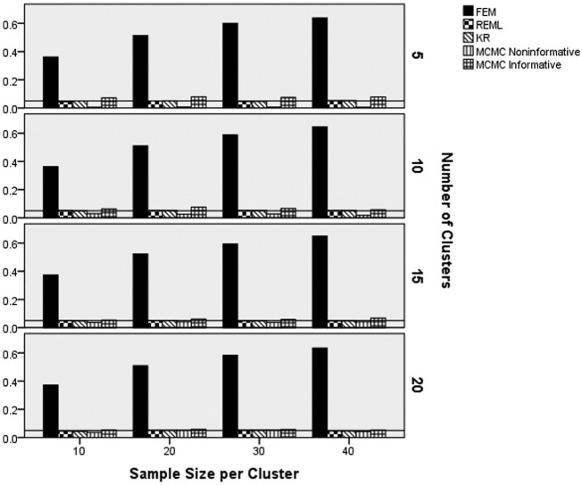
With respect to the Type I error rate of the test for the null hypothesis that the slope is 0 in the population, the interaction of estimation method by number of clusters, and sample size per cluster ($F_{36,72}=2.48,p<.001,{\eta }^2=0.55$) was statistically significant, as was the interaction of the estimation method and the slope variance ($F_{8,32}=7.22,p<.001,{\eta }^2=0.64$). Figure 7 displays the Type I error rate by estimation method, number of clusters, and sample size per cluster. A reference line has been placed at the nominal 0.05 level. FEM had an error rate exceeding the nominal 0.05 level across all number of clusters and sample size per cluster conditions. The FEM error rate increased concomitantly with increases in the sample size per cluster. The REML, KR, and noninformative MCMC methods all uniformly yielded error rates at or below the 0.05 level. The Informative MCMC estimator had Type I error rates of between 0.06 and 0.07 when the number of clusters was 5, but had values at the nominal level for 10, 15, and 20 clusters. The Type I error rate by estimation method and slope variance appears in Table 2. The error rates for REML, KR, and the noninformative MCMC estimators were all at or below the nominal 0.05 level, regardless of the slope variance. In addition, the informative MCMC estimator had error rates between 0.06 and 0.07 across conditions. Finally, FEM consistently yielded inflated Type I error rates, with higher values being associated with a larger slope variance.

Figure 7.

Type I error rate for the slope parameter by estimation method, number of clusters, and sample size per cluster.

Note. FEM = fixed effects modeling; REML = multilevel modeling using restricted maximum likelihood estimation; KR = Kenward–Rogers correction for multilevel modeling; MCMC = Markov chain Monte Carlo with informative or noninformative priors. A reference line has been placed at the nominal 0.05 level.

Table 2.

Type I Error Rate by Estimation Method and Slope Variance.

				MCMC
Slope variance	FEM	REML	KR	Noninformative	Informative
.25	.43	.05	.05	.03	.07
.50	.54	.05	.05	.03	.06
.75	.61	.05	.05	.03	.06

Note. FEM = fixed effects modeling; REML = multilevel modeling using restricted maximum likelihood estimation; KR = Kenward–Rogers correction for multilevel modeling; MCMC = Markov chain Monte Carlo with informative or noninformative priors.

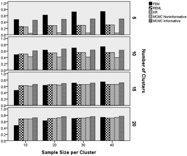
Results of the ANOVA revealed that the interactions of estimation method by slope variance and slope magnitude ($F_{36,72}=2.48,p<.001,{\eta }^2=0.55$) and estimation method by number of clusters by sample size per cluster ($F_{36,72}=2.48,p<.001,{\eta }^2=0.55$) were the two highest order terms that were statistically significantly related to power rates. All other terms were either not statistically significant or were subsumed into one of these interactions. Figure 8 includes the power for detecting a non-0 Level 1 slope by the number of clusters and the sample size per cluster. Great care must be taken when interpreting the power results of FEM, given the inflated Type I error rates that were reported above. For this reason, no further mention of the power for this approach will be made here. In terms of the other methods, as can be seen in Figure 8 (particularly for the 5 clusters case), the informative MCMC estimator yielded the highest level of power across number of clusters and sample size per cluster, though this advantage over the other estimators declined as the number of clusters and sample size per cluster increased in value. The second highest power rates for 5 and 10 clusters belonged to the REML and KR methods, with the lowest power being associated with noninformative MCMC. However, for 15 or 20 clusters the power rates of REML, KR, and the noninformative MCMC techniques were all quite similar (within 0.02 of one another), and just below those of informative MCMC.

Figure 8.

Power for the slope parameter by estimation method, number of clusters, and sample size per cluster.

Note. FEM = fixed effects modeling; REML = multilevel modeling using restricted maximum likelihood estimation; KR = Kenward–Rogers correction for multilevel modeling; MCMC = Markov chain Monte Carlo with informative or noninformative priors.

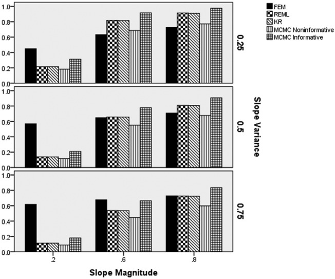
Figure 9 includes power for the slope parameter by estimation method, slope magnitude, and slope variance. As before, given its elevated Type I error rate across conditions, power results for FEM will not be interpreted here. Similar to the results reported above with respect to the number of clusters and sample size per cluster, the informative MCMC estimator yielded slightly higher power rates than did the other methods, and the noninformative MCMC had slightly lower power. Power for all methods were larger for larger slope magnitude values and for smaller slope variances.

Figure 9.

Power for the slope parameter by estimation method, slope variance, and slope magnitude.

Note. FEM = fixed effects modeling; REML = multilevel modeling using restricted maximum likelihood estimation; KR = Kenward–Rogers correction for multilevel modeling; MCMC = Markov chain Monte Carlo with informative or noninformative priors.

Summary of Coefficient Estimate Results

The preceding results demonstrated several patterns with regard to the various estimators being compared in this study. In the presence of random Level 2 variance, the MCMC-based approaches yielded the least biased estimates of the relationship between the target Level 1 predictor and the outcome variable, regardless of the combination of conditions. In addition, their estimation accuracy was largely unaffected by the number of clusters or sample size per cluster. FEM yielded the most biased slope estimate results across all conditions. In addition to yielding the most biased estimates, FEM also had the largest empirical standard errors of the methods studied here, along with the lowest coverage rates, and the most inflated Type I error rates. In terms of standard errors for the other methods, REML and KR generally had the lowest values, particularly for smaller slope magnitudes. The coverage and Type I error rates for the non-FEM estimators were all comparable to one another, and generally at or near the nominal rates that would be expected (i.e., 0.95 for coverage and 0.05 for Type I error). Finally, the noninformative MCMC estimator yielded lower power than did the other methods, particularly for smaller numbers of clusters.

Coefficient Variance Component Estimate

As with the coefficient parameter estimate itself, ANOVA was also used to identify manipulated study factors that were associated with the estimate of the slope variance. Results of the ANOVA revealed that the interaction of the estimation method, number of clusters, and sample size per cluster ($F_{18,378}=18.59,p<.001,{\eta }^2=0.47$), estimation method by number of clusters and population slope variance ($F_{12,378}=34.55,p<.001,{\eta }^2=0.52$), and estimation method by underlying model ($F_{2,188}=340.59,p<.001,{\eta }^2=0.78$) were significantly related to bias in the slope variance component estimate. Table 3 includes the bias associated with the slope variance component estimate by the estimation method, number of clusters, and sample size per cluster. The REML and KR methods had virtually identical levels of bias, which were lower than those of either MCMC estimator. The noninformative MCMC variance estimate yielded larger bias than did the other methods (noninformative MCMC variance ranging from 0.09 to 1.07 compared to <.02 for all other methods). In general, bias in the slope variance estimate declined with an increasing number of clusters. In addition, for the 15 and 20 clusters condition, bias for the REML, KR, and informative MCMC estimators declined in value as the sample size per cluster increased. However, for 5 and 10 clusters this inverse relationship between bias and sample size per cluster was not evidenced.

Table 3.

Slope Variance Estimate Bias by Estimation Method, Number of Clusters, and Sample Size per Cluster.

				MCMC
Number of clusters	Sample size per cluster	REML	KR	Noninformative	Informative
5	10	.00445	.00445	1.07610	−.02252
	20	.00615	.00615	.87950	−.02167
	30	−.00900	−.00900	.84912	−.02185
	40	−.00309	−.00309	.81296	−.02239
10	10	.00121	.00121	.29588	−.01134
	20	−.00342	−.00342	.21292	−.01577
	30	−.00037	−.00037	.21050	−.01891
	40	−.00115	−.00115	.24034	−.01865
15	10	−.00026	−.00026	.12119	−.01668
	20	−.00010	−.00010	.10756	−.01554
	30	.00167	.00167	.13098	−.00667
	40	.00034	.00034	.12706	−.00663
20	10	.00074	.00074	.08858	−.01608
	20	.00099	.00099	.09136	−.00149
	30	−.00066	−.00066	.08680	−.00083
	40	.00054	.00054	.08760	−.00021

Note. REML = multilevel modeling using restricted maximum likelihood estimation; KR = Kenward–Rogers correction for multilevel modeling; MCMC = Markov chain Monte Carlo with informative or noninformative priors.

Table 4 contains the slope variance component bias results by the number of clusters, the population slope variance value, and the estimation method. From these results, it can be seen that bias for the noninformative MCMC estimator was uniformly the highest (ranging from 0.05 to 1.30), whereas slope variance estimate bias for the REML and KR was consistently the lowest (all bias <.01). Across all estimators, the amount of bias was smaller for a larger number of clusters and increased with increasing values of the population slope variance for REML, KR, and noninformative MCMC. Table 5 includes the slope variance component estimate bias by method and underlying model. For all four estimators, the bias was greater for the model containing the Level 2 covariate (Model 2) as opposed to the simpler model without the Level 2 covariate (Model 1).

Table 4.

Slope Variance Estimate Bias by Estimation Method, Number of Clusters, and Population Slope Variance.

				MCMC
Number of clusters	Pop slope variance	REML	KR	Noninformative	Informative
5	.25	.00129	.00129	.50004	−.02523
	.50	−.00611	−.00611	.90889	−.02166
	.75	.00370	.00370	1.30433	−.01942
10	.25	−.00011	−.00011	.13153	−.01939
	.50	.00109	.00109	.24336	−.01598
	.75	−.00379	−.00379	.34483	−.01313
15	.25	.00097	.00097	.06809	−.01485
	.50	−.00195	−.00195	.11878	−.01119
	.75	.00221	.00221	.17822	−.00809
20	.25	−.00031	−.00031	.04781	−.01404
	.50	.00047	.00047	.08876	−.01222
	.75	.00106	.00106	.12918	.01231

Note. REML = multilevel modeling using restricted maximum likelihood estimation; KR = Kenward–Rogers correction for multilevel modeling; MCMC = Markov chain Monte Carlo with informative or noninformative priors.

Table 5.

Slope Variance Estimate Bias by Estimation Method and Underlying Model.

			MCMC
Model	REML	KR	Noninformative	Informative
1	.00043	.00043	.31325	−.00992
2	−.00068	−.00068	.36405	−.01723

Note. REML = multilevel modeling using restricted maximum likelihood estimation; KR = Kenward–Rogers correction for multilevel modeling; MCMC = Markov chain Monte Carlo with informative or noninformative priors. Model 1 = random coefficients multilevel model with one Level 1 predictor. Model 2 = random coefficients multilevel model with two Level 1 predictors and one Level 2 predictor.

Slope Variance Component Standard Error

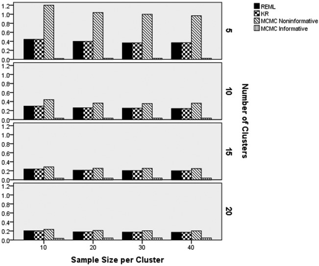
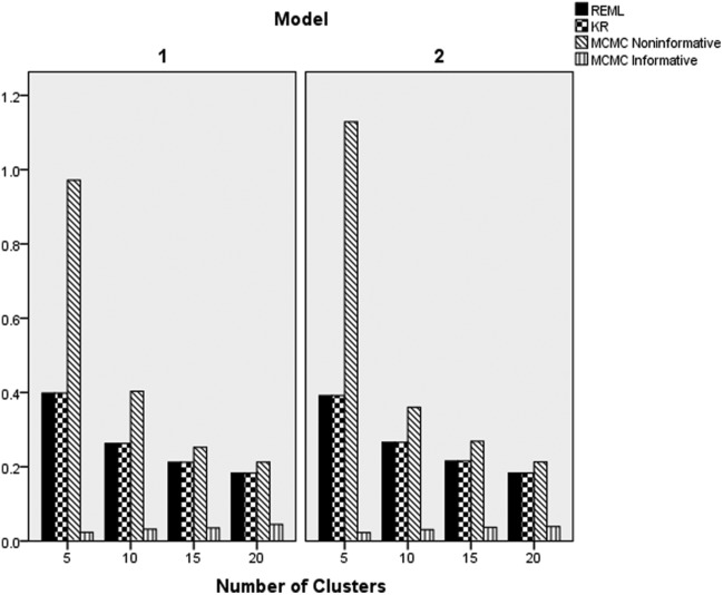
ANOVA identified the interactions of estimation method by underlying model by number of clusters ($F_{6,378}=49.04,p<.001,{\eta }^2=0.44$) and estimation method by number of clusters by sample size per cluster ($F_{18,378}=18.59,p<.001,{\eta }^2=0.47$) as the highest order statistically significant terms with respect to the magnitude of the standard error for the slope variance. Figure 10 includes the empirical standard error of the slope variance component estimate by estimation method, number of clusters, and sample size per cluster. Across conditions, the standard error of the noninformative MCMC estimator was the largest, whereas that of the informative MCMC estimator was the smallest. For all methods, the standard error declined with a larger number of clusters, and to a much smaller degree, with a larger sample size per cluster. Figure 11 displays the empirical standard error by the estimation method, the number of clusters, and the underlying model. The primary result on display in this graph is that the empirical standard error for the noninformative MCMC estimator was larger when the underlying model included a Level 2 predictor (Model 2), whereas for the other estimators there was no effect of underlying model on this outcome. As was demonstrated in Figure 10, the presence of more clusters was associated with lower standard errors for all methods, except for the informative MCMC, for which the standard error was essentially unchanged regardless of the number of clusters.

Figure 10.

Empirical standard error of random slope variance by estimation method, number of clusters, and sample size per cluster.

Note. REML = multilevel modeling using restricted maximum likelihood estimation; KR = Kenward–Rogers correction for multilevel modeling; MCMC = Markov chain Monte Carlo with informative or noninformative priors.

Figure 11.

Empirical standard error of random slope variance by estimation method, number of clusters, and underlying model.

Note. REML = multilevel modeling using restricted maximum likelihood estimation; KR = Kenward–Rogers correction for multilevel modeling; MCMC = Markov chain Monte Carlo with informative or noninformative priors. Model 1 = random coefficients multilevel model with one Level 1 predictor. Model 2 = random coefficients multilevel model with two Level 1 predictors and one Level 2 predictor.

Slope Variance Component Coverage

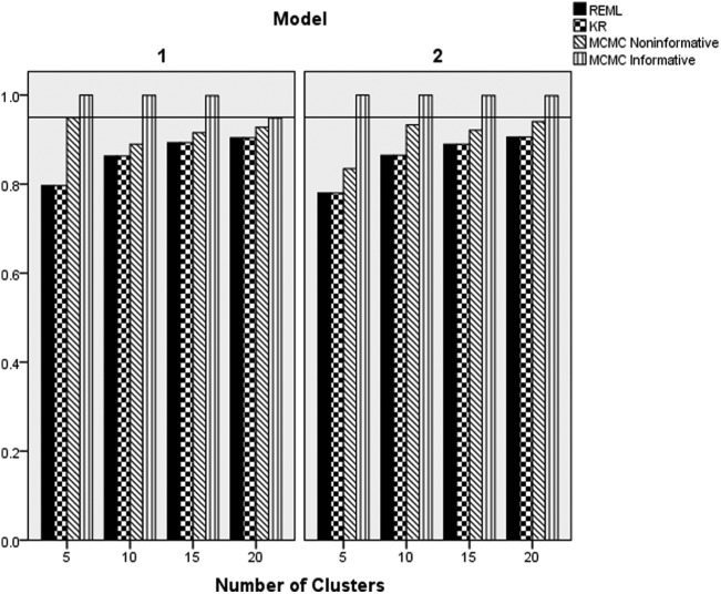
The ANOVA results identified the interaction of estimation method by Underlying Model and Number of Clusters as the highest order statistically significant term with respect to the coverage rates of the random slope variance estimate ($F_{6,378}=27.06,p<.001,{\eta }^2=0.30$). Figure 12 displays the coverage rates for this combination of conditions, with a reference line placed at the nominal 0.95 level. The only estimator that consistently had coverage rates at or above the nominal level was informative MCMC. Conversely, both REML and KR had coverage rates below the nominal level across conditions, with lower rates being associated with fewer clusters. Coverage rates for REML and KR were somewhat lower when the model included a Level 2 predictor (Model 2). Finally, the noninformative MCMC estimator yielded higher coverage rates than did either REML or KR, but lower than the informative MCMC approach.

Figure 12.

Coverage rates of random slope variance by estimation method, underlying model, and number of clusters.

Note. REML = multilevel modeling using restricted maximum likelihood estimation; KR = Kenward–Rogers correction for multilevel modeling; MCMC = Markov chain Monte Carlo with informative or noninformative priors. Model 1 = random coefficients multilevel model with one Level 1 predictor. Model 2 = random coefficients multilevel model with two Level 1 predictors and one Level 2 predictor. A reference line has been placed the nominal 0.95 level.

Slope Variance Power Rates

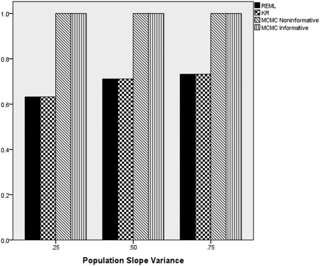
The ANOVA results revealed that the interactions of estimation method by slope variance magnitude in the population ($F_{2,189}=8932.30,p<.001,{\eta }^2=0.99$), and estimation method by number of clusters by sample size per cluster ($F_{9,189}=6921.57,p<.001,{\eta }^2=0.10$) were statistically significantly related to the power rates for the test of the null hypothesis that the slope variance is equal to 0. Figure 13 contains the power rates by the estimation method and population slope variance component magnitude. As depicted in Figure 13, both MCMC methods had higher power rates than did either REML or KR, with values for the former being 1.0 in all cases. In addition, power for REML and KR increased concomitantly with higher values of the population slope variance values.

Figure 13.

Power by estimation method and population slope variance magnitude.

Note. REML = multilevel modeling using restricted maximum likelihood estimation; KR = Kenward–Rogers correction for multilevel modeling; MCMC = Markov chain Monte Carlo with informative or noninformative priors.

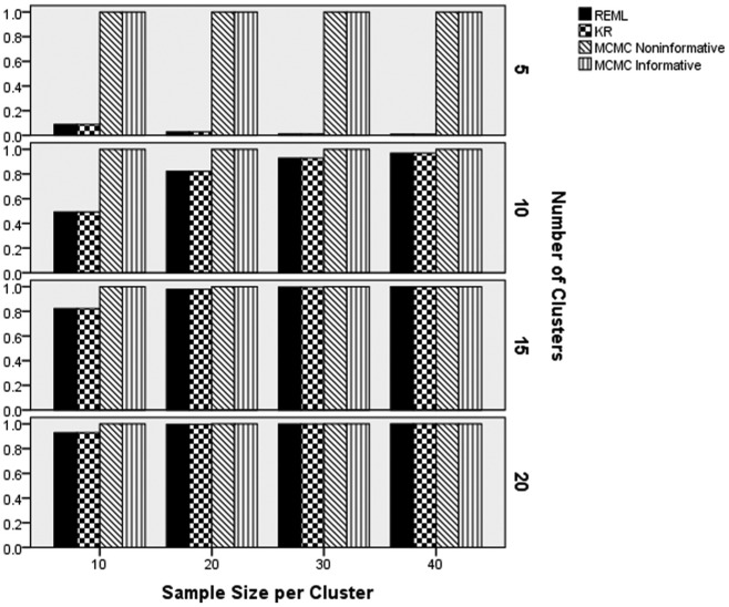
Figure 14 includes power by estimation method, number of clusters, and sample size per cluster. For five clusters, power rates for REML and KR were below 0.10, whereas those for the two MCMC estimators were 1.0. Power for REML and KR was higher for more clusters. In addition, with the exception of the 5 clusters condition, power increased for REML and KR with increased in the sample size per cluster. Finally, power rates for REML and KR were comparable to those for the two MCMC estimators in the 15 and 20 clusters conditions with 20 or more individuals per cluster.

Figure 14.

Power by estimation method, number of clusters, and sample size per cluster.

Note. REML = multilevel modeling using restricted maximum likelihood estimation; KR = Kenward–Rogers correction for multilevel modeling; MCMC = Markov chain Monte Carlo with informative or noninformative priors.

Summary of Slope Variance Estimate Results

Taken together, the results presented above demonstrated that the REML and KR estimators provide the least biased estimates of the slope variance value across conditions, whereas the largest amount of bias was associated with the noninformative MCMC estimator. In addition, all of the methods studied here yielded less biased estimates in the presence of more clusters and when the underlying model did not include a Level 2 predictor. The standard errors of the estimates were lowest for the informative MCMC estimator and highest for the noninformative MCMC. Coverage and power rates were superior for both MCMC estimators when compared with either REML or KR. Indeed, the power rates of the two MCMC methods were 1.0 across conditions.

Discussion

Several important results emerge from this set of simulations. First and foremost, results indicate that correct modeling of Level 2 slope variance is indeed important when Level 2 slope variation does exist in the population. Thus, although FEM does allow for the explanation of Level 2 variance in the dependent variable, the inability to specifically model random slope variation appears to introduce bias into the slope parameter estimates, while also increasing the empirical standard error, drastically increasing the Type I error rate, and reducing the confidence interval coverage. This result builds on the findings of McNeish and Stapleton (2016) who found that FEM used with small numbers of clusters tended to produce downward biased variance estimates and that use of REML should alleviate this issue. Taken together, these results demonstrate the importance of modeling Level 2 variation in multilevel models, particularly when samples and numbers of clusters are small. McNeish and Stapleton (2016) suggested the use of the Kenward–Rogers correction or Bayesian estimation as other potential options for small numbers of clusters. Building on this suggestion, the present study found traditional MLM using REML estimation, the Kenward–Rogers correction, and MCMC methods all to provide more favorable results than FEM, with the MCMC methods providing the least biased Level 1 coefficient estimates. It is also interesting to note that the only time model complexity arises as a statistically significant factor is when looking at slope parameter bias. For all estimation methods, slope parameter bias was larger for the more complex model (Model 2). In all other outcomes measured, however, model complexity did not factor in.

Second, when looking specifically at estimation of slope variance, MCMC with informative priors was superior to the REML and KR methods in terms of power, confidence interval coverage, and standard error. However, the MLM methods produced the least biased estimates of slope variance estimation. It is also important to note that MCMC with noninformative priors yielded the most biased results across all conditions for estimation of slope variance. This is important to consider from a practical standpoint. If a researcher is capable of using informative priors, this is obviously a very useful method for a variety of outcomes. Many fields, however (social and behavioral sciences, in particular) are likely not going to have information to generate informative priors. In these circumstances, when estimation of slope variation is desired, it appears to be more harmful to use MCMC with noninformative priors than to use a traditional MLM technique.

Third, the importance of having informative or noninformative priors for MCMC seems to depend on the outcome of interest. In terms of overall slope estimation, it did not seem to matter whether the priors were informative or not, as both methods produced similar results. However, as discussed above, with regard to estimating slope variation, noninformative priors produced the most biased results. Thus, when choosing an estimation method it is important to carefully consider your desired outcome.

Last, and not surprisingly, larger cluster size and more clusters were associated with more favorable results across conditions. Although the Kenward–Rogers correction for MLM using REML is designed to allow for smaller numbers of clusters to be used for model estimation, particularly with respect to standard errors, no differences were found for either slope parameter or slope variation estimation. Any differences in study outcomes were only apparent at the third or fourth decimal point.

Considering these results together suggests that choice of multilevel analysis technique should not be a decision based on convention or “industry standard” but rather a choice based on the following considerations:

1. The design of the model. Does the model focus on Level 1, Level 2, or a combination of both? Will the researcher be modeling random slope variation? If the focus is on Level 1 information and slopes are known (or strongly believed) not to vary among Level 2 units, then FEM may be a viable technique. However, when Level 1 coefficients do vary at Level 2 FEM is not a viable option, and MLM (i.e., REML, KR) or MCMC methods should be considered instead.

2. The purpose for the analysis. Is the researcher interested in slope parameter estimation or slope variance estimation? Is bias or power for detecting non-0 effects more important? Results of this study indicate that MLM methods tend to produce the least biased estimates for slope and slope variance parameters, but MCMC tends to yield higher power for the variance parameter estimates.

3. Information available. Does the researcher have the information necessary in order to provide accurate informative priors for Bayesian analysis? If so, then this would be the estimator of choice. If not, however, then it is important to remember that the use of noninformative priors may be detrimental to analysis, particularly for slope variance parameter estimation.

Directions for Future Research

The results of the current study suggest a number of directions that future research in the area of MLM estimation in the context of a small number of Level 2 units could take. For example, future research should continue this line of questioning to look further into the performance of FEM and MLM when the Level 2 coefficient variance value is very small, but not 0 (e.g., 0.05, 0.1). This study also set the intraclass correlation to 0.2. Although a plausible value that is representative of what is seen in practice, other values will certainly appear in applied settings. Therefore, future research should consider the impact on performance of multilevel techniques of other intraclass correlation values, both larger and smaller than 0.2. In addition, future work should examine the performance of the REML and KR methods when Level 2 coefficient variance is not 0, but the models are fit assuming it is. With regard to the MCMC estimator, future work needs to examine the impact of using incorrect informative priors on parameter estimation. In other words, if informative priors are used, and the mean is not equal to the actual parameter value, what is the impact on parameter estimation, standard errors, coverage rates, and hypothesis test results? How incorrect do the priors need to be in order to see a degradation in these outcomes? Finally, given the flexibility of FEM for modeling when researchers may not know, or have access to important Level 2 covariates, it would seem worthwhile to examine alternative methods for fitting these models that might account for the random coefficient variation that caused this approach such problems in the current study. Looking further into these methods as well as continuing to develop and promote new methods will hopefully lead to some very promising methods and recommendations for future use.

References

- Allison P. D. (2009). Fixed effects regression models. Thousand Oaks, CA: Sage. [Google Scholar]
- Asparouhov T., Muthén B. (2010). Weighted least squares estimation with missing data. Retrieved from http://www.statmodel.com/download/GstrucMissingRevision.pdf
- Bell B. A., Morgan G. B., Schoeneberger J. A., Kromrey J. D., Ferron J. M. (2014). How low can you go? An investigation of the influence of sample size and model complexity on point and interval estimates in two-level linear models. Methodology: European Journal of Research Methods for the Behavioral and Social Sciences, 10, 1-11. doi: 10.1027/1614-2241/a000062 [DOI] [Google Scholar]
- Browne W. J., Draper D. (2006). A comparison of Bayesian and likelihood-based methods for fitting multilevel models. Bayesian Analysis, 1, 473-514. doi: 10.1214/06-BA117 [DOI] [Google Scholar]
- Chaplin D. (2003). Hierarchical linear models: Strengths and weaknesses. Paper presented at the annual meeting of the Association for Public Policy Analysis and Management, Washington, DC. [Google Scholar]
- Cohen J. (1988). Statistical power analysis for the behavioral sciences. New York, NY: Routledge Academic. [Google Scholar]
- Congdon P. (2003). Applied Bayesian modeling. West Sussex, England: Wiley. [Google Scholar]
- Escobar M., Alarcon R., Blanca M. J., Fernandez-Baena F. J., Rosel J. F., Trianes M. V. (2013). Daily stressors in school-age children: A multilevel approach. School Psychology Quarterly, 28, 227-238. doi: 10.1037/spq0000020 [DOI] [PubMed] [Google Scholar]
- Ferron J. M., Bell B. A., Hess M. R., Rendina-Gobioff G., Hibbard S. T. (2009). Making treatment effect inferences from multiple-baseline data: The utility of multilevel modeling approaches. Behavior Research Methods, 41, 372-384. doi: 10.3758/BRM.41.2.372 [DOI] [PubMed] [Google Scholar]
- French B. F., Finch W. H. (2013). Extensions of Mantel-Haenszel for multilevel DIF detection. Educational and Psychological Measurement, 73, 648-671. doi: 10.1177/0013164412472341 [DOI] [Google Scholar]
- Galbraith S., Daniel J. A., Vissel B. (2010). A study of clustered data and approaches to its analysis. Journal of Neuroscience, 30, 10601-10608. doi:10.1523/JNEUROSCI .0362-10.2010 [DOI] [PMC free article] [PubMed] [Google Scholar]
- Gelman A. (2006). Prior distributions for variance parameters in hierarchical models (comment on article by Browne and Draper). Bayesian Analysis, 1, 515-534. doi: 10.1214/06-BA117A [DOI] [Google Scholar]
- Hox J. (2010). Multilevel Analysis Techniques and Applications (2nd edition) New York, NY: Routledge. [Google Scholar]
- Hox J., van de Schoot R., Matthijsse S. (2012). How few countries will do? Comparative survey analysis from a Bayesian perspective. Survey Research Methods, 6, 87-93. doi: 10.18148/srm/2012.v6i2.5033 [DOI] [Google Scholar]
- Huang F. (2016). Alternatives to multilevel modeling for the analysis of clustered data. Journal of Experimental Education, 4, 175-196. doi: 10.1080/00220973.2014.952397 [DOI] [Google Scholar]
- Kackar R. N., Harville D. A. (1984). Approximations for standard errors of estimators of fixed and random effects in mixed linear models. Journal of the American Statistical Association, 79, 853-862. doi: 10.1080/01621459.1984.10477102 [DOI] [Google Scholar]
- Kaplan D. (2014). Bayesian statistics for the social sciences. New York, NY: Guilford Press. [Google Scholar]
- Kenward M. G., Roger J. H. (2009). An improved approximation to the precision of fixed effects from restricted maximum likelihood. Computational Statistics & Data Analysis, 53, 2583-2595. doi: 10.1016/j.csda.2008.12.013 [DOI] [Google Scholar]
- Maas C. J., Hox J. J. (2005). Sufficient sample sizes for multilevel modeling. Methodology: European Journal of Research Methods for the Behavioral and Social Sciences, 1, 86-92. [Google Scholar]
- McNeish D. M., Stapleton L. M. (2016). Modeling clustered data with very few clusters. Multivariate Behavioral Research, 51, 495-518. doi: 10.1027/1614-1881.1.3.86 [DOI] [PubMed] [Google Scholar]
- McNeish D., Stapleton L. M., Silverman R. D. (2017). On the unnecessary ubiquity of hierarchical linear modeling. Psychological Methods, 22, 114-140. doi:10.1037/met0 000078 [DOI] [PubMed] [Google Scholar]
- Morgan P. L., Sideridis G. D. (2006) Contrasting the effectiveness of fluency interventions for students with or At Risk for learning disabilities: A multilevel random coefficient modeling meta analysis. Learning Disabilities Research, 21, 191-210. [Google Scholar]
- Muthén L. K., Muthén B. O. (1998-2017). Mplus user’s guide (8th ed.). Los Angeles, CA: Muthén & Muthén. [Google Scholar]
- Raudenbush S. W., Bryk A. S. (2002). Hierarchical linear models: Applications and data analysis methods (2nd ed.). Thousand Oaks: Sage. [Google Scholar]
- SAS Institute. (2015). SAS Software, Version 9.3 [Computer software]. Cary, NC: Author. [Google Scholar]
- Satterthwaite F. E. (1946). An approximate distribution of estimates of variance components. Biometrics Bulletin, 2, 110-114. Retrieved from http://www.jstor.org/stable/3002019?origin=JSTOR-pdf [PubMed] [Google Scholar]
- Schoenberger J. A. (2016). The impact of sample size and other factors when estimating multilevel logistic models. Journal of Experimental Education, 84, 373-397. doi: 10.1080/00220973.2015.1027805 [DOI] [Google Scholar]
- Setodji C. M., Shwartz M. (2013). Fixed-effect or random-effect models: What are the key inference issues? Medical Care, 51(1), 25-27. doi: 10.1097/MLR.0b013e31827a8bb0 [DOI] [PubMed] [Google Scholar]
- Snijders T. A. B., Bosker R. J. (2012). Multilevel analysis: An introduction to basic and advanced multilevel modeling (2nd ed.). Thousand Oaks, CA: Sage. [Google Scholar]
- Timmermans A. C., Kuyper H., van der Werf G. (2015). Accurate, inaccurate, or biased teacher expectations: Do Dutch teachers differ in their expectations at the end of primary education? British Journal of Educational Psychology, 85, 459-478. doi:10.1111/bjep .12087 [DOI] [PubMed] [Google Scholar]