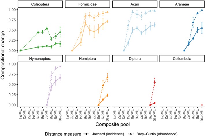
Figure 5.

Plots of compositional dissimilarity between the least‐dilute subcommunity for a taxon and subsequent subcommunities as part of more complex experimental communities. Each panel is a different taxon, and the x‐axis is experimental pools in increasing order of complexity. Y‐axis shows compositional dissimilarity, with 0 = identical and 1 = completely dissimilar (no shared OTUs). Line types show dissimilarity measure: Jaccard (presence–absence only) or Bray–Curtis (read numbers). Points and error bars show mean and standard error. Note that the leftmost point in each plot is the reference subcommunity and therefore will always have a dissimilarity value of 0