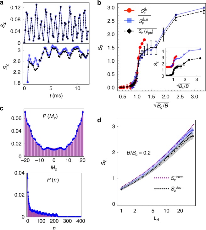
Fig. 4.

Using RE and FOTOCs to characterize chaos and thermalization in the Dicke model. a Time evolution of the spin−phonon RE $S_2\left({\widehat{\rho }}_{\mathrm{ph}}\right)$ (black lines) for the initial state ${\mid \mathrm{\Psi }}_0^{\mathrm{c}}⟩=\mid {\left(-N∕2\right)}_x⟩\otimes \mid 0⟩$ with B > B_c (top) and B < B_c (bottom). The RE is tracked excellently by the FOTOC expressions (blue lines) $S_{\mathrm{F}}^{{Ŝ}_{\mathbf{r}}}=-\log \left(I_0^{{Ŝ}_{\mathbf{r}}}\right)$ and $S_{\mathrm{F}}^{{Ŝ}_{\mathbf{r}},\widehat{n}}=-\log \left(I_0^{{Ŝ}_{\mathbf{r}}}+I_0^{\widehat{n}}\right)$ respectively. Here, ${Ŝ}_{\mathbf{r}}$ is chosen to minimize the coherence and diagonal terms in Eq. (4) (Supplementary Methods). b Long-time spin−phonon RE $S_2\left({\widehat{\rho }}_{\mathrm{ph}}\right)$ as a function of transverse field. To remove finite-size effects and residual oscillations we plot a time-averaged value $\overline{S_2\left({\widehat{\rho }}_{\mathrm{ph}}\right)}$ for 4 ms ≤  t ≤ 12 ms (FOTOC quantities are averaged identically). The regular and chaotic dynamics for the initial state ${\mid \mathrm{\Psi }}_0^{\mathrm{c}}⟩$ are clearly delineated: $\overline{S_2\left({\widehat{\rho }}_{\mathrm{ph}}\right)}\approx 0$ for B > B_c and $\overline{S_2\left({\widehat{\rho }}_{\mathrm{ph}}\right)}>0$ for B < B_c respectively. Error bars indicate standard deviation of temporal fluctuations. In the inset we plot the same FOTOC quantities but including decoherence due to single-particle dephasing at the rate Γ = 60 s⁻¹. The coherent parameters g, B and δ are enhanced by a factor of 16 compared to the main panel, as per ref. ⁶⁰. c Time-averaged distribution functions (markers) for spin-projection P(M_z) and phonon occupation P(n) (6 ms ≤ t ≤ 12 ms). We compare to the distribution of the diagonal ensemble (purple bars, see Methods). d Bipartite RE $S_2\left({\widehat{\rho }}_{L_A}\right)$ (black markers) as a function of partition size L_A of the spins, averaged over same time window as (c). For comparison, we plot the RE of a thermal canonical ensemble with corresponding temperature T fixed by the energy of the initial state ${\mid \mathrm{\Psi }}_0^{\mathrm{c}}⟩$, $S_2^{\mathrm{therm}}$ and the RE of the diagonal ensemble (see Methods). Volume-law behavior of the RE is replicated by the FOTOC quantity (blue markers). Note that the dimension of the spin Hilbert space scales linearly with L_A. Shaded regions indicate standard deviation of temporal fluctuations. Data for (a)–(d) is obtained for N = 40, with g and δ identical to calculations of Fig. 2. For (c) and (d) we choose B/(2π) = 0.7 kHz (B/B_c = 0.2). Source data are provided as a Source Data file