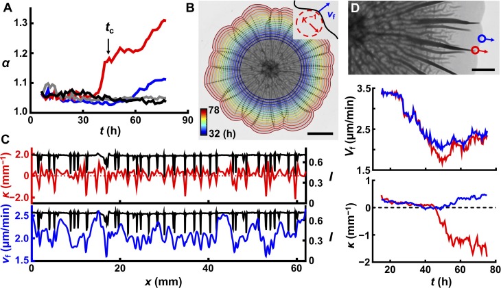
Figure 6. Delamination defines the overall biofilm contour.

(A) Time evolution of acircularity index α (where α = P²/4πA, in which P is the perimeter of the biofilm and A is the area) of the biofilm contour. Two agar substrate concentrations are shown (0.4%, red; 1.0%, blue) for WT V. cholerae biofilms. The sharp upturn in α defines the critical time t_c. Biofilms lacking matrix (ΔvpsL mutant; 0.4%, gray) or possessing an unstructured matrix (ΔrbmAΔbap1ΔrbmC mutant; 0.4%, black) remain circular. (B) Image of a WT V. cholerae biofilm grown on 0.7% agar 78 hr after inoculation, overlaid with the time evolution of the biofilm boundary. Colors correspond to the expanding boundary from 32 to 78 hr. Scale bar: 5 mm. Inset: schematic of local velocity V_f and the inverse of local curvature κ⁻¹. (C) Transmitted light intensity profiles I (black), κ (red), and V_f (blue) along the biofilm periphery from panel (B) at 60 hr. (D) Top: partial image of the biofilm shown in panel (B) at 75 hr. Red and blue dots denote two boundary points at the locations of a delaminated and a flat region, respectively. Arrows indicate boundary expansion. Middle and bottom: time evolution of V_f and κ of the designated time points during biofilm development. Scale bar: 2 mm.

Figure 6—figure supplement 1. Delamination triggers global and local slowdown of biofilm expansion and shapes the biofilm contour.

(A) Time evolution of the acircularity index α of the biofilm contour. Data are shown in magenta, blue, and black for three biofilms grown on 0.4% (solid curves) and 1.0% (dashed curves) agar plates. (B) Profiles of transmitted light intensity I (black), local curvature κ (red), and local expansion velocity V_f (blue) along the periphery of the biofilm shown in Figure 6B but at 32 hr. At 32 hr, the wrinkling/delamination pattern had not yet reached the boundary, so the biofilm remained approximately circular, and thus both I and κ remain constant over the biofilm periphery. V_f fluctuated modestly, probably because of noise at the growing front and errors in the edge tracking process. (C) Image of a WT V. cholerae biofilm grown on 0.7% agar taken 30 hr after inoculation. R_f and R_p denote the radius of the entire biofilm (outlined in red) and the distal radius to which the morphological pattern extends (outlined in blue), respectively. Scale bar: 2 mm. (D) Time evolution of R_f (solid curves) and R_p (dashed curves). Data are shown from three different WT V. cholerae biofilms (denoted by different colors) grown on 0.4% agar. Initially, R_p lags behind R_f, indicating a peripheral zone in which the biofilm remains flat and lacks identifiable features. R_f increases linearly with time, which defines an expansion velocity <V_f> . At a critical time t’_c (35 hr (black), 42.5 hr (blue), and 45 hr (magenta) for the three cases shown), the region harboring wrinkles or blisters rapidly propagates to the edge of the biofilm (R_p = R_f). Concurrently, the global biofilm expansion velocity slows, with a crossover time point at t’_c. Inset: close-up view of R_f and R_p versus time for one set of data (blue) around t’_c. The critical time that is defined in this manner matches that defined from the α – t plot in Figure 6A (i.e. t_c = t’_c), suggesting that mechanical instability at the biofilm edge triggers the development of contour undulations. (E) Averaged biofilm expansion velocity <V_f> before (white) and after (gray) morphological features appear at the rim. <V_f> was calculated by linear fitting of R_f versus time. Data are represented as mean ± std with n = 3.

Figure 6—figure supplement 2. Blister formation drives the overall biofilm contour.

(A) (Left) Bright-field image of a typical 60-hr-old biofilm growing on an agar substrate with predefined defects. The eight surface defects (marked by red crosses) trigger the formation of blisters, which subsequently define the positions of eight ‘petals’ along the biofilm contour. (B) (Left) Transmission image of a 40-hr-old biofilm grown in a line geometry on an agar substrate. Red outlines indicate the upper and bottom contours. (Right) Analyses identical to that provided in Figure 6C were performed for both contours to show that the formation of blisters (indicated by the valleys in the intensity profiles(black)) locally slows down biofilm expansion velocity (blue) and defines the indentation positions along the contour (red). Scale bars: 5 mm.