Monotone FISTA with Variable Acceleration for Compressed Sensing Magnetic Resonance Imaging

Abstract

An improvement of the monotone fast iterative shrinkage-thresholding algorithm (MFISTA) for faster convergence is proposed. Our motivation is to reduce the reconstruction time of compressed sensing problems in magnetic resonance imaging. The proposed modification introduces an extra term, which is a multiple of the proximal-gradient step, into the so-called momentum formula used for the computation of the next iterate in MFISTA. In addition, the modified algorithm selects the next iterate as a possibly-improved point obtained by any other procedure, such as an arbitrary shift, a line search, or other methods. As an example, an arbitrary-length shift in the direction from the previous iterate to the output of the proximal-gradient step is considered. The resulting algorithm accelerates MFISTA in a manner that varies with the iterative steps. Convergence analysis shows that the proposed modification provides improved theoretical convergence bounds, and that it has more flexibility in its parameters than the original MFISTA. Since such problems need to be studied in the context of functions of several complex variables, a careful extension of FISTA-like methods to complex variables is provided.

I. Introduction

Magnetic Resonance Imaging (MRI) is a versatile modality for qualitative and quantitative imaging of the human body [1]. However, data acquisition usually requires a long scan time. Compressed sensing (CS) [2, 3] can be deployed to reduce this time. CS uses undersampled data and sparsity promoting reconstruction, achieving almost exactly the same image quality as the reconstructions with fully sampled data, but with much faster acquisition. Several important MRI applications [4] became more efficacious by using CS. For example, CS can increase spatiotemporal resolution while reducing motion-related artifacts in dynamic MRI [4] and can reduce the necessary time for data acquisition in quantitative mapping applications up to 10 times [5], with very small mapping error.

Image reconstruction in MRI using CS (CS-MRI) can be posed as an optimization problem defined over complex vectors x ∈ ℂⁿ; that is vectors with complex components. We consider problems of the following kind: Find an x* that minimizes

$$\mathrm{\Psi }(\text{x})=f(\text{x})\hspace{0.17em}+\hspace{0.17em}\varphi (\text{x}),$$ (1)

where f : ℂⁿ → ℝ is convex, continuously differentiable and satisfies $\Vert \nabla f(\text{x})-\nabla f(\text{y})\Vert <\mathcal{L}\Vert \text{x}-\text{y}\Vert$ for some constant $\mathcal{L}\in ℝ$ (such an $\mathcal{L}$ is referred to as a Lipschitz constant for the gradient ∇f), while ϕ : ℂⁿ → ℝ is also convex, but may be nonsmooth. Here $\Vert \text{x}\Vert$ denotes the Euclidean norm of x. Definitions and notation used here and elsewhere in this paper are summarized in the Appendix, based on material in [6].

In the context of CS-MRI problems $f(\text{x})=\frac{1}{2}{\Vert g-\mathbf{A}\text{x}\Vert }^2$ where the vector x ∈ ℂⁿ represents the images, the vector g ∈ ℂ^m represents the captured k-space data, and the transform A represent the system matrix (described in more detail in the experimental Section V). The choice for the second (regularization) function in (1) is usually the ℓ₁-norm of a transformed version of x [3, 7], such as $\varphi (\text{x})=\lambda \Vert \mathbf{T}\text{x}{\Vert }_1$, or a low-rank imposing nuclear-norm [8, 9], such as $\lambda {\Vert \text{x}\Vert }_{\ast }$, or a combination of both, such as in low-rank plus sparse decomposition [5, 10].

The reconstruction time, i.e. the computation time to minimize (1), is extremely important in CS-MRI applications. In particular for radial and other non-Cartesian MRI (and similar problems with ill-conditioned system matrices), fast algorithms able to deal with non-differentiability of ϕ(x) are required. The proximal-gradient methods can deal with non-differentiability of ϕ(x). These methods make use of a proximal-gradient step (with step-size 1/L):

$$P_L(\text{y}):=\underset{\varphi ,\hspace{0.17em}L}{\text{prox}}\left(\text{y}-\frac{1}{L}\nabla f(\text{y})\right),$$ (2)

where

$$\underset{\varphi ,\hspace{0.17em}L}{\text{prox}}(\text{x}):=\underset{\text{z}\in {ℂ}^n}{\text{arg min}}\left\{\varphi (\text{z})+\frac{L}{2}{\Vert \text{z}-\text{x}\Vert }^2\right\},$$ (3)

is the proximal operator [11] of ϕ for parameter L ∈ ℝ.

It was almost a decade ago when the proximal-gradient methods called fast iterative shrinkage-thresholding algorithms (FISTA) and monotone FISTA (MFISTA) were proposed by Beck and Teboulle [7, 12]. (Other proximal-gradient algorithms appeared in the optimization literature even earlier, in particular in the context of image processing [13, 14].) These methods successfully combine a proximal-gradient step [11, 15] with a so-called momentum step as suggested in [16] to obtain fast convergence satisfying the following (based on theorems from [7, 12]): Let $L\ge \mathcal{L}$, x_k denote the k-th iterate generated by FISTA or MFISTA with constant parameter L in the proximal operator, and let x^∗ be any minimizer of the Ψ in (1), then it is the case that

$$\mathrm{\Psi }({\text{x}}_k)-\mathrm{\Psi }({\text{x}}^{\ast })\le \frac{2L{\Vert {\text{x}}_0-{\text{x}}^{\ast }\Vert }^2}{{(k+1)}^2}.$$ (4)

In [17], Kim and Fessler modified FISTA inspired by the Performance Estimation Problems (PEP) technique [18], with practical improvement in convergence. They named the algorithm optimized ISTA (OISTA), due to its similarity to their optimized gradient method (OGM) for smooth functions in [19]. For OGM, in the convergence result that corresponds to (4), the upper bound is reduced by a factor of 2, but no such a bound is known for OISTA. Recently, a new version of the fast and optimal proximal-gradient methods, with a similar bound, appeared in [20]. Another practical way to accelerate FISTA and obtain monotonicity is by restarting FISTA when $\mathrm{\Psi }({\text{x}}_k)<\mathrm{\Psi }({\text{x}}_{k+1})$, as shown in [21].

However, theoretical convergence speed can, in fact, be improved over (4) by more than the factor 2 suggested in [17, 19]. Our main contribution in the present paper is the introduction of an algorithm with a convergence upper bound such that the L in the right-hand side of (4) is replaced by $L_k/{\eta }_k$ where L_k may be smaller than $\mathcal{L}$ and/or η_k may be larger than 1. The L_k may be known before algorithm execution, but the η_k is not; it is calculated during the execution of the k-th iterative step of the new algorithm (see Step 7 of Algorithm 2 below). The η_k is then used in the calculation of the multiplier of the proximal-gradient step in the extra term in the momentum formula (see Step 8 of Algorithm 2); it is in this sense that the new algorithm uses “variable acceleration.” We will see that in practice the obtained convergence bound for the new algorithm is very often less than half of the right-hand side of (4) and it can be proven that the upper bound is no larger than the right-hand side of (4). A similar method is the overrelaxed MFISTA (OMFISTA) [22], which also uses an extra term in the momentum formula and variable step-size L_k. Our proposed method goes further by taking advantage of gaps in the relations used in the convergence analysis and converting them into larger η_k, resulting in faster convergence.

In Section II the MFISTA algorithm is reviewed. In Section III the proposed revisited version of MFISTA is presented, and its convergence analysis is provided in Section IV. Some experimental results illustrating convergence performance on compressed sensing for MRI problems are shown in Section V. A discussion is presented in Section VI, and a summary is provided in Section VII.

II. Review of MFISTA

The version of MFISTA that we use in this paper to minimize (1) is specified in Algorithm 1, with the following parameters: x₀ (the initial iterate), N (the number of iterations) and a sequence (L₁, …, L_N) of positive real numbers (that determine the step-sizes $1/L_k$ to be used in the iterative steps).

As an example, with the $f(\text{x})=\frac{1}{2}{\Vert \text{g}-\text{Ax}\Vert }^2$ and with $\varphi (\text{x})=\lambda {\Vert \text{x}\Vert }_1$, the proximal-gradient operator computed in Step 4 of Algorithm 1 becomes (see [12, 23]):

$$P_{L_k}({\text{y}}_k):=S_{\lambda /L_k}(\frac{1}{L_k}{\text{A}}^{†}(\text{g}-\text{A}{\text{y}}_k)+{\text{y}}_k),$$ (5)

where A^† is the adjoint of A (see [6, (A.4)]) and S_α, the shrinkage-thresholding operator, is defined for any given

$$\begin{array}{l}\mathbf{\text{Algorithm}}\hspace{0.17em}\hspace{0.17em}\mathbf{1}\hspace{0.17em}\text{MFISTA}\\ \hspace{0.17em}\hspace{0.17em}1:\hspace{0.17em}\hspace{0.17em}\mathbf{\text{set}}\hspace{0.17em}{t}_1=1\\ \hspace{0.17em}\hspace{0.17em}2:\hspace{0.17em}\hspace{0.17em}\mathbf{\text{set}}\hspace{0.17em}{\text{y}}_1={\text{x}}_0\\ \hspace{0.17em}\hspace{0.17em}3:\hspace{0.17em}\hspace{0.17em}\mathbf{\text{for}}\hspace{0.17em}k=1\hspace{0.17em}\text{to}\hspace{0.17em}N\hspace{0.17em}\mathbf{\text{do}}\\ \hspace{0.17em}\hspace{0.17em}4:\hspace{0.17em}\hspace{0.17em}\hspace{0.17em}\hspace{0.17em}\hspace{0.17em}\mathbf{\text{set}}\hspace{0.17em}{\text{z}}_k=P_{L_k}({\text{y}}_k)\\ \hspace{0.17em}\hspace{0.17em}5:\hspace{0.17em}\hspace{0.17em}\hspace{0.17em}\hspace{0.17em}\hspace{0.17em}\mathbf{\text{set}}\hspace{0.17em}{\text{x}}_k=\underset{\text{x}\in {\{\text{z}}_k{\text{,x}}_{k-1}\}}{\text{arg min}}\hspace{0.17em}\hspace{0.17em}\mathrm{\Psi }(\text{x})\\ \hspace{0.17em}\hspace{0.17em}6:\hspace{0.17em}\hspace{0.17em}\hspace{0.17em}\hspace{0.17em}\hspace{0.17em}\mathbf{\text{set}}\hspace{0.17em}{t}_{k+1}=(1+\sqrt{1+4t_k^2})/2\\ \hspace{0.17em}\hspace{0.17em}7:\hspace{0.17em}\hspace{0.17em}\hspace{0.17em}\hspace{0.17em}\hspace{0.17em}\mathbf{\text{set}}\hspace{0.17em}{\text{y}}_{k+1}={\text{x}}_k+\frac{t_{k-1}}{t_{k+1}}({\text{x}}_k-{\text{x}}_{k-1})+\frac{t_k}{t_k+1}({\text{z}}_k-{\text{x}}_k)\\ \hspace{0.17em}\hspace{0.17em}8:\hspace{0.17em}\hspace{0.17em}\mathbf{\text{end}}\hspace{0.17em}\mathbf{\text{for}}\end{array}$$

complex vector u = (u₁, …, u_N)^T and real number α by: S_α(u) = (v₁, …, v_N)^T, with

$$v_n=\{\begin{array}{ll}0\hfill & ,\hspace{0.17em}\text{if}\hspace{0.17em}\left|u_n\right|<\alpha ,\hfill \\ u_n-\alpha \frac{u_n}{\left|u_n\right|}\hfill & ,\hspace{0.17em}\text{otherwise}.\hfill \end{array}$$ (6)

When the nuclear-norm $\varphi (\text{x})=\lambda {\Vert \text{x}\Vert }_{\ast }$ is used, the shrinkage-thresholding is still part of the proximal operator [8], but it is applied on the singular values of the Casorati matrix constructed with the vector x [10].

Compared to algorithms like FISTA, MFISTA introduces an extra computation of the cost function, as shown in Step 5 of Algorithm 1. For CS-MRI applications, the costs of the operations Ax or A^†x are extremely high, and such is required by FISTA and MFISTA. For this reason, efficient implementations that reuse these operations for computing the cost function are essential for achieving computation times for each iteration that are similar to those of FISTA.

III. The Proposed Improvement to MFISTA

The purpose of this section is to indicate the ideas that lead us to the algorithm MFISTA with Variable Acceleration (MFISTA-VA) that we claim to be an improvement over MFISTA. First we state, in Algorithm 2, a mathematically precise specification of MFISTA-VA. This is followed by an informal discussion of the algorithm. A mathematically rigorous analysis of the convergence properties of the algorithm is provided in the next section.

$$\begin{array}{l}\mathbf{\text{Algorithm}}\hspace{0.17em}\hspace{0.17em}2\hspace{0.17em}\text{MFISTA-VA}\\ \hspace{0.17em}\hspace{0.17em}1:\hspace{0.17em}\hspace{0.17em}\mathbf{\text{set}}\hspace{0.17em}{t}_1=1\\ \hspace{0.17em}\hspace{0.17em}2:\hspace{0.17em}\hspace{0.17em}\mathbf{\text{set}}\hspace{0.17em}{\text{y}}_1={\text{x}}_0\\ \hspace{0.17em}\hspace{0.17em}3:\hspace{0.17em}\hspace{0.17em}\mathbf{\text{for}}\hspace{0.17em}k=1\hspace{0.17em}\text{to}\hspace{0.17em}N\hspace{0.17em}\mathbf{\text{do}}\\ \hspace{0.17em}\hspace{0.17em}4:\hspace{0.17em}\hspace{0.17em}\hspace{0.17em}\hspace{0.17em}\hspace{0.17em}\mathbf{\text{set}}\hspace{0.17em}{\text{z}}_k=P_{L_k}({\text{y}}_k)\\ \hspace{0.17em}\hspace{0.17em}5:\hspace{0.17em}\hspace{0.17em}\hspace{0.17em}\hspace{0.17em}\hspace{0.17em}\mathbf{\text{set}}\hspace{0.17em}{\text{x}}_k=\underset{\text{x}\in \{{\overline{\text{x}}}_k,z_k,x_{k-1}\}}{\text{arg min}}\hspace{0.17em}\hspace{0.17em}\mathrm{\Psi }(\text{x})\\ \hspace{0.17em}\hspace{0.17em}6:\hspace{0.17em}\hspace{0.17em}\hspace{0.17em}\hspace{0.17em}\hspace{0.17em}\mathbf{\text{set}}\hspace{0.17em}{t}_{k+1}=\left(1+\sqrt{1+4t_k^2}\right)/2\\ \hspace{0.17em}\hspace{0.17em}7:\hspace{0.17em}\hspace{0.17em}\hspace{0.17em}\hspace{0.17em}\hspace{0.17em}\mathbf{\text{set}}\hspace{0.17em}{\eta }_k=1+2\frac{Q_{L_k}({\text{z}}_k,{\text{y}}_k)-\mathrm{\Psi }({\text{x}}_k)}{L_k{\Vert {\text{z}}_k-{\text{y}}_k\Vert }^2}\\ \hspace{0.17em}\hspace{0.17em}8:\hspace{0.17em}\hspace{0.17em}\hspace{0.17em}\hspace{0.17em}\hspace{0.17em}\mathbf{\text{set}}\hspace{0.17em}{\text{y}}_{k+1}={\text{x}}_k+\frac{t_{k-1}}{t_{k+1}}({\text{x}}_k-{\text{x}}_{k-1})+\frac{t_k}{t_{k+1}}({\text{z}}_k-{\text{x}}_k)+\\ \hspace{0.17em}\hspace{0.17em}\hspace{0.17em}\hspace{0.17em}\hspace{0.17em}\hspace{0.17em}\hspace{0.17em}\hspace{0.17em}\hspace{0.17em}\hspace{0.17em}\frac{t_k}{t_{k+1}}({\eta }_k-1)({\text{z}}_k-{\text{y}}_k)\\ \hspace{0.17em}\hspace{0.17em}9:\hspace{0.17em}\hspace{0.17em}\mathbf{\text{end}}\hspace{0.17em}\mathbf{\text{for}}\end{array}$$

Both MFISTA and MFISTA-VA share the same step ${\text{z}}_k=P_{L_k}({\text{y}}_k)$ (Step 4 of MFISTA in Algorithm 1, and Step 4 of MFISTA-VA in Algorithm 2). This step arises from the minimization of the quadratic surrogate Q_L(z, y) (seen in Step 7 of Algorithm 2) that is defined, for L ∈ ℝ and z, y ∈ ℂⁿ,as:

$$Q_L(\text{z,}\hspace{0.17em}\text{y})\hspace{0.17em}:=f(\text{y})+\Re (\langle \nabla f(\text{y}),\text{z}-\text{y}\rangle )+\frac{L}{2}{\Vert \text{z}-\text{y}\Vert }^2+\varphi (\text{z}),$$ (7)

where both the gradient ∇ and the scalar product ⟨⟩ are to be interpreted as the complex ones; see (53)–(56) of the Appendix. However, one of the major convergence conditions of FISTA and MFISTA is

$$\mathrm{\Psi }({\text{z}}_k)\le Q_{L_k}(z_k,{\text{y}}_k).$$ (8)

Note that if $L\ge \mathcal{L}$, then Ψ(z) ≤ Q_L (z, y) for all z, y ∈ ℂⁿ, as can be derived from [12, Lemma 2.1]), using (54) and (56) of the A This implies that any step-size $1/L_k$ longer than $1/\mathcal{L}$, in FISTA or MFISTA, requires (8) to be satisfied. That condition, together with L_k ≤ L_k+1 from [12, Lemma 4.1]), limits the convergence speed of FISTA and MFISTA.

In the revisited convergence analysis of the next section, (8) is relaxed. There (see Lemma 3) we take advantage of the gap

$${\zeta }_k\hspace{0.17em}:=Q_{L_k}({\text{z}}_k,{\text{y}}_k)-\mathrm{\Psi }({\text{z}}_k)$$ (9)

between the surrogate and the cost function to replace (8) by the weaker convergence condition

$$1+2\frac{{\zeta }_k}{L_k{\Vert {\text{z}}_k-{\text{y}}_k\Vert }^2}>0,$$ (10)

guaranteeing algorithm convergence with proximal-gradient steps with step-size $1/L_k$ in (2) larger than what was allowed by (8). Note that the gap ζ_k can be negative, in which case (8) is not satisfied for the chosen L_k. However, this is not necessarily a problem in the new algorithm, as long as (10) is satisfied, as seen further in the next section.

The gap ζ_k is easily computed. In fact, due to (7) and (1):

$$\begin{gathered} {\zeta }_k=Q_{L_k}({\text{z}}_k,{\text{y}}_k)-\mathrm{\Psi }({\text{z}}_k) \\ =f({\text{y}}_k)+\Re (\langle \nabla f({\text{y}}_k),{\text{z}}_k-{\text{y}}_k\rangle )-f({\text{z}}_k) \\ \hspace{1em}\hspace{1em}\hspace{1em}\hspace{1em}\hspace{1em}\hspace{1em}\hspace{1em}\hspace{1em}\hspace{1em}\hspace{1em}\hspace{1em}+\frac{L_k}{2}{\Vert {\text{z}}_k-{\text{y}}_k\Vert }^2, \end{gathered}$$ (11)

which does not depend on ϕ, but depends on f.

In addition, we may use line search such as in [24, 25], or any rule that give us a point x_k not worse than z_k, in the sense Ψ(x_k) ≤ Ψ(z_k), to further accelerate the algorithm. With this idea in mind, at Step 5 of the proposed MFISTA-VA method, described in Algorithm 2, we introduce an arbitrary point ${\overline{\text{x}}}_k$ that will be chosen to be the current iterate x_k instead of the proximal-gradient z_k or the previous iterate x_k−1, which are the only choices in Step 5 of MFISTA (Algorithm 1), if $\mathrm{\Psi }({\overline{\text{x}}}_k)$ is the smallest value in the set $\{\mathrm{\Psi }({\overline{\text{x}}}_k),\mathrm{\Psi }(x_{k-1}),\mathrm{\Psi }(z_k)\}$. In our experiments reported in Section V we use ${\overline{\text{x}}}_k={\text{x}}_{k-1}+\mu ({\text{z}}_k-{\text{x}}_{k-1})$, where the coefficient μ is a user-selected parameter. This choice of ${\overline{\text{x}}}_k$ is similar to the one used in OMFISTA, however, according to [22, Theorem 1], only μ ≤ 1 is allowed in OMFISTA.

When MFISTA-VA obtains Ψ(x_k) ≤ Ψ(z_k), it generates the extra gap (always nonnegative)

$${\delta }_k=\mathrm{\Psi }({\text{z}}_k)-\mathrm{\Psi }({\text{x}}_k)$$ (12)

which is then used with ζ_k to compute the parameter

$${\eta }_k\hspace{0.17em}:=1+2\frac{{\zeta }_k+{\delta }_k}{L_k{\Vert {\text{z}}_k-{\text{y}}_k\Vert }^2},$$ (13)

used in Step 8 of Algorithm 2. The extra gap δ_k had never been exploited before, and may produce a large η_k, improving the convergence speed as clarified in what follows.

Proposition 1. Let x₀ ∈ ℂⁿ, N be a positive integer, (L₁, …, L_N) be a sequence of positive real numbers, x_k, y_k, z_k and η_k be the sequences generated by Algorithm 2. For 1 ≤ k ≤ N, if (10) is satisfied, then η_k > 0.

Proof: The sum of the positive left hand side of (10) and an appropriately selected nonnegative multiple of the nonnegative right hand side of (12) is in fact η_k. ■

Theorem 5 of the next section guarantees the following convergence speed result for MFISTA-VA: If x^∗ is a minimizer of the Ψ in (1), then

$$\mathrm{\Psi }({\text{x}}_k)-\mathrm{\Psi }({\text{x}}^{\ast })\le \frac{2L_k{\Vert {\text{x}}_0-{\text{x}}^{\ast }\Vert }^2}{{\eta }_k{(k+1)}^2},$$ (14)

provided that $L_k/{\eta }_k\le L_{k+1}/{\eta }_{k+1}$, for 1 ≤ k < N. We remark that this monotonicity condition for the ratios L_k/η_k makes the mathematical expression for the convergence bound simpler, but we conjecture that similar convergence results still hold under less stringent conditions.

By using (12) and (9) in (13), we have

$${\eta }_k=1+2\frac{Q_{L_k}({\text{z}}_k,{\text{y}}_k)-\mathrm{\Psi }({\text{x}}_k)}{L_k{\Vert {\text{z}}_k-{\text{y}}_k\Vert }^2}.$$ (15)

Note that if $\mathrm{\Psi }({\text{z}}_k)\le Q_{L_k}({\text{z}}_k,{\text{y}}_k)$ then (15) implies η_k ≥ 1. Therefore, by comparing (4) with (14) we conclude that if, in addition, L_k ≤ L, then MFISTA-VA has a better theoretical convergence bound than FISTA and MFISTA. The improvement in the theoretical convergence bound is by a factor η_k, that can be larger than 2 in practice. This is not always guaranteed to be the case, however, since it depends on ζ_k and δ_k, which in turn depend on the chosen L_k and the procedure that yields ${\overline{\text{x}}}_k$. For example, if L_k is such that $\mathrm{\Psi }({\text{z}}_k)=Q_{L_k}({\text{z}}_k,{\text{y}}_k)$ and if x_k is such that $\mathrm{\Psi }({\text{x}}_k)=\mathrm{\Psi }({\text{z}}_k)$, then we have η_k = 1 and thus the last term $\frac{t_k}{t_{k+1}}({\eta }_k-1)\hspace{0.17em}({\text{z}}_k-{\text{y}}_k)$ on the right-hand side of the assignment in Step 8 of Algorithm (2) has no effect. In this case our proposed algorithm reduces itself to FISTA and the convergence bound reduces itself to the same as for FISTA.

The convergence bound in (14) is better when the ratio $L_k/{\eta }_k$ is small, that is, when L_k is small and/or when η_k is large. Unfortunately, when the user-defined parameter L_k decreases, the η_k returned by Step 7 of Algorithm 2 also decreases. A search procedure for Lk that minimizes $L_k/{\eta }_k$ is not always a viable option, because it potentially requires multiple computations of the proximal-gradient operator, which is the time-consuming operation of the algorithm. Here, the introduction of the ${\overline{\text{x}}}_k$ makes a difference, by obtaining good ratios $L_k/{\eta }_k$ without resorting to costly operations. This new variable gives to the proposed algorithm more flexibility and the potential to be even faster. The ${\overline{\text{x}}}_k$ may be obtained by any other algorithm or procedure, such as line search, arbitrary shifts or other combination of previous iterates. According to Step 5 of Algorithm 2, if $\mathrm{\Psi }({\overline{\text{x}}}_k)$ reduces the cost function more than $\mathrm{\Psi }({\text{z}}_k)$ or $\mathrm{\Psi }({\text{x}}_{k-1})$, it will be chosen as $\mathrm{\Psi }({\text{x}}_k)$, increasing η_k and, consequently improving the ratio $L_k/{\eta }_k$.

IV. Convergence Analysis

In this section we provide a mathematical convergence analysis of the proposed algorithm. We start with a mathematical proposition that is relevant to all proximal-gradient methods. After that we state and prove the key Lemma 3, which will be used to prove our Theorem 5 on the rate of convergence.

Proposition 2. Let y be in ℂⁿ and let L be a positive real number. Let f, ϕ and P_L be as defined in (1) and (2) and let ϕ′ (P_L(y)) be a subgradient of ϕ at P_L(y); see (59). Then

$$\nabla f(\text{y})+\varphi \text{'}(P_L(\text{y}))=-L(P_L(\text{y})-\text{y}).$$ (16)

Proof: As stated after (59) in the Appendix, z is a minimizer of F : ℂⁿ → ℝ if, and only if, the zero vector 0 is a subgradient of F at z. Considering (2) and (3), let

$$P_L(\text{y})=\underset{\text{z}\in {ℂ}^n}{\text{arg min}}\left\{\varphi (\text{z})+\frac{L}{2}{\Vert \text{z}-\left(\text{y}-\frac{1}{L}\nabla f(\text{y})\right)\Vert }^2\right\}.$$ (17)

The proposition follows from the material after (59) in the Appendix. ■

Lemma 3. Let L be a positive real number. Let Ψ, f, ϕ, P_L and Q_L be as defined in (1), (2) and (7). Let y, u ∈ ℂⁿ and ζ, δ ∈ ℝ be defined by

$$\zeta =Q_L(P_L(\text{y}),\text{y})-\mathrm{\Psi }(P_L(\text{y}))$$ (18)

and

$$\delta =\mathrm{\Psi }(P_L(\text{y}))-\mathrm{\Psi }(\text{u}).$$ (19)

Then, for every x ∈ ℂⁿ,

$$\begin{gathered} \mathrm{\Psi }(\text{x})-\mathrm{\Psi }(\text{u})\ge \frac{L}{2}{\Vert P_L(\text{y})-\text{y}\Vert }^2 \\ \hspace{1em}\hspace{1em}\hspace{1em}\hspace{1em}\hspace{1em}\hspace{0.17em}+L\Re (\langle P_L(\text{y})-\text{y},\text{y}-\text{x}\rangle )+\zeta +\delta . \end{gathered}$$ (20)

Further,

$$\begin{gathered} \mathrm{\Psi }(\text{x})-\mathrm{\Psi }(\text{u})\ge \frac{\eta L}{2}{\Vert P_L(\text{y})-\text{y}\Vert }^2 \\ \hspace{1em}\hspace{1em}\hspace{1em}\hspace{1em}\hspace{1em}\hspace{0.17em}+L\Re (\langle P_L(\text{y})-\text{y},\text{y}-\text{x}\rangle ), \end{gathered}$$ (21)

with

$$\eta =1+\frac{\zeta +\delta }{\frac{L}{2}{\Vert P_L(\text{y})-\text{y}\Vert }^2}.$$ (22)

Proof: Since f is convex and differentiable we get that

$$f(\text{y})\le f(\text{x})+\Re (\langle \nabla f(\text{y}),\text{y}-\text{x}\rangle ),$$ (23)

see (58) in the Appendix, and

$$\varphi (P_L(\text{y}))\le \varphi (\text{x})+\Re (\langle \varphi \text{'}(P_L(\text{y})),P_L(\text{y})-\text{x}\rangle ),$$ (24)

for any x, y ∈ ℂⁿ, where ϕ′ (w) is a subgradient of ϕ at w, see (59) in the Appendix. Now, because of (18), from (9) and (7) with z = P_L(y) we have

$$\begin{gathered} \mathrm{\Psi }(P_L(\text{y}))=f(\text{y})+\Re (\langle \nabla f(\text{y}),P_L(\text{y})-\text{y}\rangle ), \\ \hspace{1em}\hspace{1em}\hspace{1em}\hspace{1em}\hspace{1em}\hspace{1em}+\frac{L}{2}{\Vert P_L(\text{y})-\text{y}\Vert }^2+\varphi (P_L(\text{y}))-\zeta . \end{gathered}$$ (25)

Therefore, after including (23) and (24),

$$\begin{gathered} \mathrm{\Psi }(P_L(\text{y}))\le \\ \hspace{1em}\hspace{1em}f(\text{x})+\Re (\langle \nabla f(\text{y})+\varphi \text{'}(P_L(\text{y})),P_L(\text{y})-\text{x}\rangle ) \\ \hspace{1em}\hspace{1em}\hspace{1em}\hspace{1em}\hspace{1em}\hspace{1em}\hspace{1em}+\frac{L}{2}{\Vert P_L(\text{y})-\text{y}\Vert }^2+\varphi (\text{x})-\zeta . \end{gathered}$$ (26)

After using (16), we get

$$\begin{gathered} \mathrm{\Psi }(\text{x})-\mathrm{\Psi }(P_L(\text{y}))\ge \Re (\langle L(P_L(\text{y})-\text{y}),P_L(\text{y})-\text{x}\rangle ) \\ \hspace{1em}\hspace{1em}\hspace{1em}\hspace{1em}\hspace{1em}\hspace{1em}\hspace{1em}\hspace{1em}\hspace{1em}\hspace{1em}-\frac{L}{2}{\Vert P_L(\text{y})-\text{y}\Vert }^2+\zeta . \end{gathered}$$ (27)

and then

$$\begin{array}{l}\mathrm{\Psi }(\text{x})-\mathrm{\Psi }(P_L(\text{y}))\ge L\Re (\langle P_L(\text{y})-\text{y},\text{y}-\text{x}\rangle )\\ \hspace{1em}\hspace{1em}\hspace{1em}\hspace{1em}\hspace{1em}\hspace{1em}\hspace{1em}\hspace{1em}\hspace{1em}\hspace{1em}+\frac{L}{2}{\Vert P_L(\text{y})-\text{y}\Vert }^2+\zeta .\end{array}$$ (28)

Using (19) this leads to (20), proving the first part of Lemma 3. The second part. which is in (21), follows trivially. ■

We note that Lemma 3 is quite general; it does not depend on the algorithm chosen to solve the optimization problem.

Proposition 4. Let x₀ ∈ ℂⁿ, N be a positive integer, (L₁, …, L_N) be a sequence of positive real numbers, x_k, y_k, z_k and η_k be the sequences generated by Algorithm 2. Consider a fixed integer $\overline{k}$, $1\le \overline{k}\le N$. In Lemma 3, let $L=L_{\overline{k}}$, $\text{y}={\text{y}}_{\overline{k}}$, $\text{u}={\text{x}}_{\overline{k}}$ and define ζ and δ so that (18) and (19) hold. Then, for any choice of x in Lemma 3, the η of (22) is equal to ${\eta }_{\overline{\text{k}}}$.

Proof: This follows immediately from (18), (19) and Steps 4 and 7 of Algorithm 2. ■

Theorem 5. Let x₀ ∈ ℂⁿ, x* be a minimizer of the Ψ in (1), N be a positive integer, (L₁, …, L_N) be a sequence of positive real numbers, x_k, y_k, z_k and η_k be the sequences generated by Algorithm 2 such that, for 1 ≤ k ≤ N, (10) is satisfied. Then, for 1 ≤ k ≤ N, (14) holds provided that L_k/η_k ≤ L_k+1/η_k+1 for 1 ≤ k < N and

$$\mathrm{\Psi }({\text{x}}_k)-\mathrm{\Psi }({\text{x}}^{\ast })\le \frac{2L_1{\Vert {\text{x}}_0-{\text{x}}^{\ast }\Vert }^2}{{\eta }_1{(k+1)}^2}$$ (29)

holds provided that L_k/η_k ≥ L_k+1/η_k+1 for 1 ≤ k < N.

Proof: Let k be a fixed integer, 1 ≤ k < N. In Lemma 3, let L = L_k+1, y = y_k+1, u = x_k+1 and define ζ and δ so that (18) and (19) hold. With these assignments, we restate below versions of (21) of Lemma 3 for two different choices of x ∈ ℂⁿ. By Proposition 4, for any choice of x, the η of (22) is equal to η_k+1.

Our first choice is x = x_k. Using Step 4 of Algorithm 2,

$$\begin{gathered} \frac{2}{L_{k+1}}(d_k-d_{k+1})\ge {\eta }_{k+1}{\Vert {\text{z}}_{k+1}-{\text{y}}_{k+1}\Vert }^2 \\ \hspace{1em}\hspace{1em}\hspace{1em}\hspace{1em}\hspace{1em}\hspace{0.17em}\hspace{0.17em}+2\Re (\langle {\text{z}}_{k+1}-{\text{y}}_{k+1},{\text{y}}_{k+1}-{\text{x}}_k\rangle ), \end{gathered}$$ (30)

where d_k := Ψ(x_k) − Ψ(x*). Note that d_k ≥ 0.

Our second choice is x = x*, which leads to

$$\begin{gathered} \frac{2}{L_{k+1}}(-d_{k+1})\ge {\eta }_{k+1}{\Vert {\text{z}}_{k+1}-{\text{y}}_{k+1}\Vert }^2 \\ \hspace{1em}\hspace{1em}\hspace{1em}\hspace{1em}\hspace{1em}\hspace{0.17em}\hspace{0.17em}+2\Re (\langle {\text{z}}_{k+1}-{\text{y}}_{k+1},{\text{y}}_{k+1}-{\text{x}}^{\ast }\rangle ). \end{gathered}$$ (31)

Multiplying (30) and (31) by t_k+1(t_k+1 − 1) and t_k+1, respectively, and then adding the results, we get

$$\begin{gathered} \frac{2}{L_{k+1}}\left((t_{k+1}^2-t_{k+1})d_k-t_{k+1}^2{d}_{k+1}\right)\ge \\ \hspace{1em}\hspace{1em}\hspace{1em}\hspace{1em}\hspace{0.17em}\hspace{0.17em}{\eta }_{k+1}{t}_{k+1}^2{\Vert {\text{z}}_{k+1}-{\text{y}}_{k+1}\Vert }^2+ \\ 2\Re \left(\langle t_{k+1}{\text{(z}}_{k+1}-{\text{y}}_{k+1}),t_{k+1}{\text{y}}_{k+1}-(t_{k+1}-1){\text{x}}_k-{\text{x}}^{\ast }\rangle \right). \end{gathered}$$ (32)

Considering that $t_{k+1}(t_{k+1}-1)=t_k^2$ is satisfied, due to Step 6 of Algorithm 2, this results in

$$\begin{gathered} \frac{2}{L_{k+1}}\left(t_k^2{d}_k-t_{k+1}^2{d}_{k+1}\right)\ge {\eta }_{k+1}{t}_{k+1}^2{\Vert {\text{z}}_{k+1}-{\text{y}}_{k+1}\Vert }^2+ \\ 2\Re \left(\langle t_{k+1}({\text{z}}_{k+1}-{\text{y}}_{k+1}),t_{k+1}{\text{y}}_{k+1}-(t_{k+1}-1){\text{x}}_k-{\text{x}}^{\ast }\rangle \right). \end{gathered}$$ (33)

Now, we apply the easily-derivable relationship:

$$\Re (\langle \text{x},\text{y}\rangle )=\frac{1}{2\eta }\left({\Vert \eta \text{x}+\text{y}\Vert }^2-{\Vert \eta \text{x}\Vert }^2-{\Vert \text{y}\Vert }^2\right),$$ (34)

to obtain

$$\begin{gathered} \frac{2}{L_{k+2}}\left(t_k^2{d}_k-t_{k+1}^2{d}_{k+1}\right)\ge {\eta }_{k+1}{t}_{k+1}^2{\Vert {\text{z}}_{k+1}-{\text{y}}_{k+1}\Vert }^2 \\ \hspace{1em}\hspace{1em}\hspace{0.17em}\hspace{0.17em}+\frac{1}{{\eta }_{k+1}}\Vert {\eta }_{k+1}{t}_{k+1}({\text{z}}_{k+1}-{\text{y}}_{k+1}) \\ \hspace{1em}\hspace{1em}\hspace{0.17em}\hspace{1em}{+t_{k+1}{\text{y}}_{k+1}-\left(t_{k+1}-1\right){\text{x}}_k-{\text{x}}^{\ast }\Vert }^2 \\ \hspace{1em}\hspace{1em}\hspace{0.17em}\hspace{1em}\hspace{1em}-\frac{1}{{\eta }_{k+1}}{\Vert {\eta }_{k+1}{t}_{k+1}({\text{z}}_{k+1}-{\text{y}}_{k+1})\Vert }^2 \\ \hspace{1em}\hspace{1em}\hspace{0.17em}-\frac{1}{{\eta }_{k+1}}{\Vert t_{k+1}{\text{y}}_{k+1}-(t_{k+1}-1){\text{x}}_k-{\text{x}}^{\ast }\Vert }^2. \end{gathered}$$ (35)

In order to simplify the calculations, denote, for 1 ≤ k ≤ N,

$${\text{v}}_k:=t_k(1-{\eta }_k)\hspace{0.17em}{\text{y}}_k-(t_k-1){\text{x}}_{k-1}.$$ (36)

Then, the equation in Step 8 of Algorithm 2 can be written as

$$t_{k+1}{\text{y}}_{k+1}={\eta }_k{t}_k{\text{z}}_k+(t_{k+1}-1){\text{x}}_k+{\text{v}}_k.$$ (37)

This way we can rewrite (35), rearranging the elements, as

$$\begin{gathered} \frac{2}{L_{k+1}}\left(t_k^2{d}_k-t_{k+1}^2{d}_{k+1}\right)\ge \\ \hspace{1em}\hspace{1em}\hspace{0.17em}\hspace{0.17em}+\frac{1}{{\eta }_{k+1}}{\Vert {\eta }_{k+1}{t}_{k+1}{\text{z}}_{k+1}+{\text{v}}_{k+1}-{\text{x}}^{\ast }\Vert }^2 \\ \hspace{1em}\hspace{1em}\hspace{0.17em}\hspace{0.17em}\hspace{1em}\hspace{1em}\hspace{0.17em}\hspace{1em}\hspace{1em}-\frac{1}{{\eta }_{k+1}}{\Vert {\eta }_k{t}_k{\text{z}}_k+{\text{v}}_k-{\text{x}}^{\ast }\Vert }^2. \end{gathered}$$ (38)

Since 0 < η_k+1,

$$\frac{2{\eta }_{k+1}}{L_{k+1}}\left(t_k^2{d}_k-t_{k+1}^2{d}_{k+1}\right)\ge {\Vert {\text{u}}_{k+1}\Vert }^2-{\Vert {\text{u}}_k\Vert }^2,$$ (39)

with ${\text{u}}_k={\eta }_k{t}_k{\text{z}}_k+{\text{v}}_k-{\text{x}}^{\ast }$.

Assuming $L_k/{\eta }_k\le L_{k+1}/{\eta }_{k+1}$, we got (for 1 ≤ k < N)

$$\frac{2{\eta }_k{t}_k^2{d}_k}{L_k}-\frac{2{\eta }_{k+1}{t}_{k+1}^2{d}_{k+1}}{L_{k+1}}\ge {\Vert {\text{u}}_{k+1}\Vert }^2-{\Vert {\text{u}}_k\Vert }^2.$$ (40)

We work our way to proving (14) by noting that its left hand side is d_k. To get an upper bound, we rewrite (40) as a_k − a_k+1 ≥ b_k+1 − b_k and note that, consequently, a_k ≤ a₁ + b₁, for all k ≥ 1 (this is stated as Lemma 4.2 in [12]) .

In Lemma 3 and Proposition 4, let x = x*, u = x₁, y = y₁, L = L₁ and define ζ and δ so that (18) and (19) hold. Then

$$\begin{gathered} \mathrm{\Psi }({\text{x}}^{\ast })-\mathrm{\Psi }({\text{x}}_1)\ge \frac{{\eta }_1{L}_1}{2}{\Vert {\text{z}}_1-{\text{y}}_1\Vert }^2 \\ \hspace{1em}\hspace{1em}\hspace{1em}\hspace{1em}\hspace{1em}\hspace{1em}\hspace{1em}\hspace{1em}\hspace{0.17em}\hspace{0.17em}+L_1\Re \left(\langle {\text{z}}_1-{\text{y}}_1,{\text{y}}_1-{\text{x}}^{\ast }\rangle \right). \end{gathered}$$ (41)

Using (34)

$$\begin{gathered} \mathrm{\Psi }({\text{x}}^{\ast })-\mathrm{\Psi }({\text{x}}_1)\ge \frac{{\eta }_1{L}_1}{2}{\Vert {\text{z}}_1-{\text{y}}_1\Vert }^2 \\ \hspace{1em}\hspace{1em}\hspace{1em}\hspace{1em}+\frac{L_1}{2{\eta }_1}{\Vert {\eta }_1{\text{z}}_1+(1-{\eta }_1)\hspace{0.17em}{\text{y}}_1-{\text{x}}^{\ast }\Vert }^2 \\ \hspace{1em}\hspace{1em}\hspace{1em}-\frac{L_1}{2{\eta }_1}{\Vert {\eta }_1({\text{z}}_1-{\text{y}}_1)\hspace{0.17em}\Vert }^2-\frac{L_1}{2{\eta }_1}{\Vert ({\text{y}}_1-{\text{x}}^{\ast })\hspace{0.17em}\Vert }^2. \end{gathered}$$ (42)

Therefore

$$\begin{array}{l}{d}_1=\mathrm{\Psi }({\text{x}}_1)-\mathrm{\Psi }({\text{x}}^{\ast })\le \frac{L_1}{2{\eta }_1}{\Vert {\text{y}}_1-{\text{x}}^{\ast }\Vert }^2\\ \hspace{1em}\hspace{1em}\hspace{1em}\hspace{1em}\hspace{1em}\hspace{1em}-\frac{L_1}{2{\eta }_1}{\Vert {\eta }_1{\text{z}}_1+(1-{\eta }_1)\hspace{0.17em}{\text{y}}_1-{\text{x}}^{\ast }\Vert }^2.\end{array}$$ (43)

Expanding a_k ≤ a₁ + b₁, we get (for 1 ≤ k < N) that

$$\frac{2{\eta }_k{t}_k^2{d}_k}{L_k}\le \frac{2{\eta }_1{t}_1^2{d}_1}{L_1}+{\Vert {\eta }_1{t}_1{\text{z}}_1+{\text{v}}_1-{\text{x}}^{\ast }\Vert }^2.$$ (44)

Steps 1 and 2 of Algorithm 2 joined with (36) and (43) yield

$$d_k\le \frac{L_k\Vert {\text{x}}_0-{\text{x}}^{\ast }{\Vert }^2}{2{\eta }_k{t}_k^2}.$$ (45)

It is easy to prove, based on Step 6 of Algorithm 2, that t_k ≥ (k + 1) /2 (this is stated as Lemma 4.2 in [12]), which leads us to the desired result in (14).

Following the alternative path, we assume that $L_k/{\eta }_k\ge L_{k+1}/{\eta }_{k+1}$ for 1 ≤ k < N. In that case,

$$t_k^2{d}_k-t_{k+1}^2{d}_{k+1}\ge \frac{L_{k+1}}{2{\eta }_{k+1}}{\Vert {\text{u}}_{k+1}\Vert }^2-\frac{L_k}{2{\eta }_k}{\Vert {\text{u}}_k\Vert }^2.$$ (46)

Invoking Lemma 4.2 of [12], and this time considering (46) as a_k − a_k+1 ≥ b_k+1 − b_k, we have that a_k ≤ a₁ + b₁ for every k ≥ 1.

Again, t₁ = 1, but now a₁ = Ψ(x₁) − Ψ(x*) and $b_1=\left(L_1/2{\eta }_1\right)\Vert {\eta }_1{\text{z}}_1+\left(1-{\eta }_1\right){\text{y}}_1-{\text{x}}^{\ast }\Vert$, then (41) leads to

$$\begin{gathered} a_1=\mathrm{\Psi }({\text{x}}_1)-\mathrm{\Psi }({\text{x}}^{\ast })\le \frac{L_1}{2{\eta }_1}{\Vert {\text{y}}_1-{\text{x}}^{\ast }\Vert }^2 \\ \hspace{1em}\hspace{1em}\hspace{1em}\hspace{1em}\hspace{1em}\hspace{1em}-\frac{L_1}{2{\eta }_1}{\Vert {\eta }_1{\text{z}}_1+\left(1-{\eta }_1\right){\text{y}}_1-{\text{x}}^{\ast }\Vert }^2, \end{gathered}$$ (47)

and $a_1+b_1\le c=\left(L_1/2{\eta }_1\right){\Vert {\text{x}}_0-{\text{x}}^{\ast }\Vert }^2$, due to y₁= x₀. Now, t_k ≥ (k + 1) /2 gives the desired result in (29). ■

V. Experiments

In the present section, we compare the performance of the discussed algorithms when applied to specific problems of (sparse) MRI reconstruction. We note, however, that they are also applicable to reconstruction problems for other modalities of (sparse) data collection, for example by the Brazilian Synchrotron Light Source [25].

We used $f(\text{x})=\frac{1}{2}{\Vert \text{g}-\text{Ax}\Vert }^2$, where the vector x ∈ ℂⁿ represents the dynamic images, with n = N_x×N_y×N_t, where N_x is the horizontal image size, N_y is the vertical image size, and N_t is the number of time points of the imaging sequence. The vector g ∈ ℂ^m represents the captured radial k-space, originally with size m = N_s×N_r×N_c×N_t, where N_s is the number of samples on each radial k-space line, N_r is the number of radial lines, or spokes, and N_c is the number of receive coils. The transform A = SFC is composed of the multiple coil sensitivities C, which is a (N_x×N_y×N_t)×(N_x×N_y×N_c×N_t) mapping, the Fourier transforms F, for all coils, and the compressed sensing sampling pattern S. For radial or other non-Cartesian CS MRI problems, SF is a (N_x×N_y×N_c×N_t)×(N_s×N_r×N_c×N_t) mapping, performed by the undersampled Non-Uniform Fast Fourier Transform (NUFFT) [26].

The acquisition of MR images for T_1ρ (spin–lattice relaxation time in the rotating frame) mapping requires a long scan time [5, 27]. Undersampling the k-space data coupled with parallel acquisition and CS reconstruction algorithms can greatly reduce acquisition time. Because even the undersampled data acquisition process will take some non-negligible time, patient movement can happen and radial sampling of the k-space may increase the robustness of the process.

We applied MFISTA-VA to the reconstruction of two CSMRI problems for which data were originally captured with golden angle radial stack of stars [28] in 3D k-space. In these problems, data were fully sampled in the stacking direction, and were separated into 2D k-space slices by 1D IFFT (Inverse Fast Fourier Transform). After this, the 2D slices were reconstructed independently. The central area of the 2D undersampled k-space was reconstructed with NUFFT gridding [29] at a lower resolution and used for coilmap estimation, using ESPIRiT [30]. The regularization parameter λ, used as in $\varphi (\text{x})=\lambda {\Vert \text{x}\Vert }_{\ast }$ or $\varphi (\text{x})=\lambda {\Vert \text{Tx}\Vert }_1$, was manually chosen for the best visual results in both of the MRI problems that are presented next. The experiments were executed on a computer with Intel Xeon E5–2603v4 @1.7GHz, 48GB RAM. The implementation of MFISTA-VA for these CS-MRI problems, that reused the operation Ay or A^†y is presented in Algorithm 3. Note however, this implementation requires more memory since it uses extra variables. The implementation of MFISTA, FISTA and OISTA are simplified versions of it. In order to see the contributions of ${\overline{\text{x}}}_k$ or η_k separated, we included a modified version of MFISTA (no effect of η_k) and MFISTA-VA with μ = 1.0 (no effect of ${\overline{\text{x}}}_k$). The modified MFISTA has the Line 5 of Algorithm 1 replaced by Line 5 of Algorithm 2. This version (denoted mod. MFISTA in the figures) illustrates the benefits of using only ${\overline{\text{x}}}_k$. MFISTA-VA with μ = 1.0 forces ${\overline{\text{x}}}_k={\text{z}}_k$, so one can see the effect of using only ηk (however, acording to Section III, we have no contribution of the extra gap δ_k in (13)). The Matlab codes of these experiments are available online at http://cai2r.net/resources/software/cs-mri-mfista-va-matlab-code.

a). MRI Problem A:

Ten sets of 3D data of the knee were captured with a 15-channel knee coil, with 128 radial spokes (256 samples each) with golden angle increments [28], and 64 slices each, resulting in the size N_s×N_r×N_c×N_t = 256×128×15×10 after separation of the 3D data into multiple 2D slices. A 6-fold undersampling was retrospectively done for the CS tests, undersampled data is of size N_s×N_r×N_c×N_t = 256×22×15×10. This data consists of 10 T_1ρ-weighted 2D k-space sets with spin-lock times 2/4/6/8/10/15/25/35/45/55ms, similar to what was presented in [5]. The total acquisition time of the fully-sampled data is around 30 min. The CS image sequences (2D slices + time) were reconstructed using the low-rank imposing nuclear-norm [8, 9], defined by $\varphi (\text{x})=\lambda {\Vert \text{x}\Vert }_{\ast }$, with image sequence size of n = N_x×N_y×N_t = 160×160×10, and were subsequently used for T_1ρ fitting [5, 27], after reconstruction.

Two versions of the proposed MFISTA-VA, using ${\overline{\text{x}}}_k={\text{x}}_{k-1}+\mu ({\text{z}}_k-{\text{x}}_{k-1})$ with two constant coefficients μ = 1.0 and μ = 1.5, are compared with FISTA [12], MFISTA [7] and OISTA [17]. All methods utilize the same constant L_k = 30, which satisfies (8) in all iterations for convergence. A modified MFISTA, using ${\overline{\text{x}}}_k={\text{x}}_{k-1}+\mu ({\text{z}}_k-{\text{x}}_{k-1})$, with μ = 1.5 is also shown. In Figures 1 through 4, the convergence of these six algorithms is illustrated for Problem A. In Figures 1 and 2, the convergence of the cost function Ψ(x_k) − Ψ(x^∗) is shown over iteration index and time, where x^∗ is assumed to be the convergence limit.¹ In Figures 3 and 4, the distance $\Vert {\text{x}}_k-{\text{x}}^{\ast }\Vert /\Vert {\text{x}}^{\ast }\Vert$, to x^∗ is shown, over iteration and over time. In Figure 7, some visual results for the first of the 10 T_1ρ-weighted images are shown.

Figure 1:

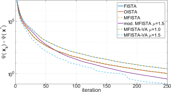
Curves showing the cost function Ψ(x_k) − Ψ(x*) over iteration index, for MRI Problem A.

Figure 4:

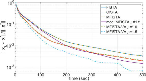
Curves showing the error $\Vert {\text{x}}_k-{\text{x}}^{\ast }\Vert /\Vert {\text{x}}^{\ast }\Vert$ over time, for MRI Problem A.

Figure 2:

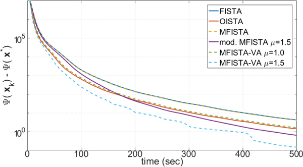
Curves showing the cost function Ψ(x_k) − Ψ(x*) over time, for MRI Problem A.

Figure 3:

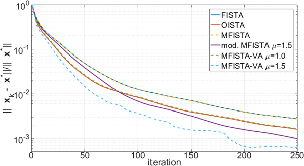
Curves showing the error $\Vert {\text{x}}_k-{\text{x}}^{\ast }\Vert /\Vert {\text{x}}^{\ast }\Vert$ over iteration index, for MRI Problem A.

Figure 7:

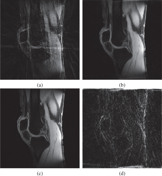
Visual example showing the first image of the reconstructed sequence of T_1ρ-weighted images of MRI Problem A. (a) NUFFT gridding of the 6-fold undersampled data (22 spokes/image), (b) MFISTA-VA of the 6-fold undersampled data, (c) NUFFT gridding of the fully sampled data (128 spokes/image), and (d) magnitude of the difference, with intensity amplified 10×, between MFISTA-VA and fully-sampled gridding.

The improvement in convergence speed of MFISTA-VA (with μ = 1.5) over FISTA, MFISTA and OISTA is clear. For MFISTA-VA with coefficient μ = 1.0 we observed that 1.426 ≤ η_k ≤ 1.997 with median value of 1.994. However, for MFISTA-VA with coefficient μ = 1.5, we observed that 1.534 ≤ η_k ≤ 12.081 with median value of 2.254. The modified MFISTA (with μ = 1.5) performed well at the final iterations, but it was slow in the initial iterations.

(b). MRI Problem B:

One 3D dataset of the liver was captured with a 20-channel abdominal coil with 128 spokes (384 samples each) with golden angle increments [28], and 88 slices, resulting in the size N_s×N_r×N_c×N_t = 384×128×20×1 after separation of the 3D data into multiple 2D slices. A 1.6-fold undersampling was retrospectively done, undersampled data is of size N_s×N_r×N_c×N_t = 384×80×20×1. In this problem the regularization is $\varphi (\text{x})=\lambda {\Vert \text{Tx}\Vert }_1$, which is the ℓ₁-norm of the first-order spatial finite difference transform, as T. This penalty is an anisotropic Total Variation (TV) penalty. In the implementation the proximal operator, in (2), was calculated using 25 iterations of the fast gradient projected algorithm [7]. The image matrix size is n = N_x×N_y×N_t = 160×320×1.

Two versions of the proposed MFISTA-VA, with two coefficients μ = 1.0 and μ = 1.5, were compared with the same methods as in the previous experiment. All methods utilized the same constant L_k = 60, which satisfies (8) in all iterations for this problem. Here, only the distance to x^∗, i.e. $\Vert {\text{x}}_k-{\text{x}}^{\ast }\Vert /\Vert {\text{x}}^{\ast }\Vert$, is shown, over iteration and over time, in Figures 5 and 6, respectively. In Figure 9 some visual results are shown. In this example, for MFISTA-VA with coefficient μ = 1 we observed that 1.356 ≤ η_k ≤ 1.993 with median value of 1.991, while with coefficient μ = 1.5 we observed that 1.480 ≤ η_k ≤ 3.197 with median value of 1.996.

Figure 5:

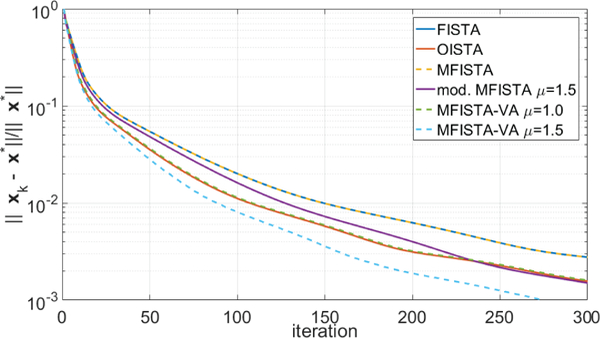
Curves showing the error $\Vert {\text{x}}_k-{\text{x}}^{\ast }\Vert /\Vert {\text{x}}^{\ast }\Vert$ over iteration index, for MRI Problem B.

Figure 6:

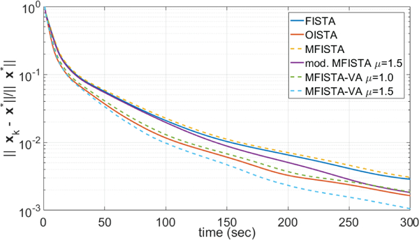
Curves showing the error $\Vert {\text{x}}_k-{\text{x}}^{\ast }\Vert /\Vert {\text{x}}^{\ast }\Vert$ over time, for MRI Problem B.

Figure 9:

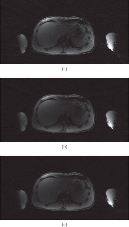
Visual example showing the reconstructed abdominal images, obtained using the l₁-norm of the first-order spatial finite difference transform regularization. (a) NUFFT gridding of the 1.6-fold undersampled data (80 spokes), (b) MFISTAVA of the 1.6-fold undersampled data, and (c) NUFFT gridding of the fully sampled data (128 spokes).

We also illustrate with an experiment the initial motivation of this work, namely, the possibility of using proximal-gradient steps $1/L_k$ larger than allowed by previously existing theory. This may also be interesting either when the Lipschitz constant for the gradient of f is not known or not easy to compute. In Problem B, the constant step L_k = 60 satisfied(8) in every iteration of all methods, thereby simultaneously honoring theoretical sufficient convergence for each of the algorithms. However, as we illustrate in Figure 8 using the convergence of the cost function difference Ψ(x_k) − Ψ(x^∗), when a smaller L_k = 40 is used, some methods may no longer converge. In this example, OISTA diverged after the 4^th iteration with L_k = 40, and FISTA diverged after the 11^th iteration. The proposed method converged with L_k = 40 (0.678 ≤ η_k ≤ 1.091, with median value of 0.722). The proposed method MFISTA-VA performed well, being more robust to the decrease in the value of L_k, and faster than FISTA and OISTA with the same L_k. Running the algorithms again starting from a small L_k, and increasing it while checking that the convergence conditions (8) and (10) are satisfied, revealed that the lower bounds for L_k were: FISTA L_k ≥ 48, OISTA L_k ≥ 58, and MFISTA-VA L_k ≥ 30.

Figure 8:

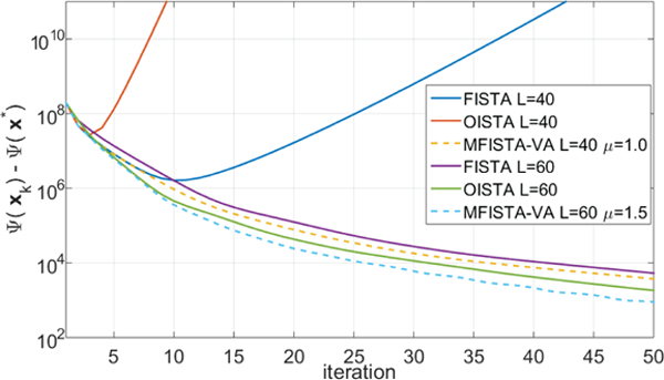
Curves showing the cost function Ψ(x_k) − Ψ(x*) over iteration for MRI Problem B, for two different L values.

VI. Discussion

As mentioned in Section III, the inclusion of the ${\overline{\text{x}}}_k$ can help to improve the convergence ratio $L_k/{\eta }_k$ by increasing η_k. The ${\overline{\text{x}}}_k$ can be obtained by any method, procedure or algorithm. It can be used even to merge the proposed FISTA-like method synergistically with other algorithms for minimizing (1), similar to what was done in [31]. What really matters is that the computational saving due to the more rapid decrease of the cost function $\mathrm{\Psi }({\overline{\text{x}}}_k)$ surpasses the computational cost of obtaining ${\overline{\text{x}}}_k$ and computing $\mathrm{\Psi }({\overline{\text{x}}}_k)$ (recall that decreasing Ψ improves the convergence ratio $L_k/{\eta }_k$). To see how this can affect positively the convergence, note that in the experiments for Problem A, a maximum η_k of 12.08 was obtained.

In this paper we report only on experiments using algorithms with the simple choice of ${\overline{\text{x}}}_k={\text{x}}_{k-1}+{\mu }_k({\text{z}}_k-{\text{x}}_{k-1})$. The increase in computational cost is small in this case, see Algorithm 3 for details, but the approach is advantageous if good values for μ_k are know. Previous experience with line search for MFISTA in [25] indicates that 1 ≤ μ_k ≤ 2 is usually a reasonable guess, but this largely depends on the application, system matrix, and choice of other parameters of the algorithm, such as L_k. Empirically, we observe that small step-sizes 1/Lk can be compensated by large coefficients μ_k. However, it is beyond the scope of this paper explore optimal values for all the parameters of the algorithm.

If x_k = z_k, which is the case in FISTA and OISTA, then δ_k = 0 in (12) and, according (13), η_k reduces to

$$\begin{gathered} {\eta }_k=1+\frac{{\zeta }_k}{\frac{L_k}{2}{\Vert {\text{z}}_k-{\text{y}}_k\Vert }^2}= \\ \hspace{1em}\hspace{1em}2+\frac{f({\text{y}}_k)-\Re \left(\langle \nabla f({\text{y}}_k),\hspace{0.17em}{\text{z}}_k-{\text{y}}_k\rangle \right)-f({\text{z}}_k)}{\frac{L_k}{2}{\Vert {\text{z}}_k-{\text{y}}_k\Vert }^2}. \end{gathered}$$ (48)

Since f is convex and differentiable, it follows from (58) of the Appendix that the numerator of the second fraction in the formula above is not positive and so η_k ≤ 2. As compared with this, in MFISTA-VA we may select an ${\overline{\text{x}}}_k$ resulting in $\mathrm{\Psi }({\text{x}}_k)=\mathrm{\Psi }({\overline{\text{x}}}_k)<\mathrm{\Psi }({\text{z}}_k)$. This results in the δ_k of (12) being positive and may result in the η_k of (13) being greater than 2. That such larger-than-two values occur in practice can be seen from the results reported in the section on Experiments. See Table I for a comparison of the convergence formulas for FISTA/MFISTA, OGM and MFISTA-VA.

Table I:

Convergence results:

Method:	Formula:
FISTA/MFISTA [7, 12]	$\mathrm{\Psi }({\text{x}}_k)-\mathrm{\Psi }({\text{x}}^{\ast })\le \frac{2L{\Vert {\text{x}}_0-{\text{x}}^{\ast }\Vert }^2}{{\left(k+1\right)}^2}$
OGM [19] (not proved for OISTA)	$\mathrm{\Psi }({\text{x}}_k)-\mathrm{\Psi }({\text{x}}^{\ast })\le \frac{L{\Vert {\text{x}}_0-{\text{x}}^{\ast }\Vert }^2}{{\left(k+1\right)}^2}$
MFISTA-VA	$\mathrm{\Psi }({\text{x}}_k)-\mathrm{\Psi }({\text{x}}^{\ast })\le \frac{2L_k{\Vert {\text{x}}_0-{\text{x}}^{\ast }\Vert }^2}{{\eta }_k{\left(k+1\right)}^2}$

$$\begin{array}{l}\mathbf{\text{Algorithm}}\hspace{0.17em}\hspace{0.17em}3\hspace{0.17em}\text{MFISTA-VA}\hspace{0.17em}\text{for}\hspace{0.17em}\text{CS-MRI}\\ \hspace{0.17em}\hspace{0.17em}1:\hspace{0.17em}\hspace{0.17em}\mathbf{\text{set}}\hspace{0.17em}{t}_1=1\\ \hspace{0.17em}\hspace{0.17em}2:\hspace{0.17em}\hspace{0.17em}\mathbf{\text{set}}\hspace{0.17em}{\text{y}}_1={\text{x}}_0\\ \hspace{0.17em}\hspace{0.17em}3:\hspace{0.17em}\hspace{0.17em}\mathbf{\text{set}}\hspace{0.17em}{\tilde{\text{y}}}_1=\text{A}{\text{x}}_0\\ \hspace{0.17em}\hspace{0.17em}4:\hspace{0.17em}\hspace{0.17em}\mathbf{\text{for}}\hspace{0.17em}k=1\hspace{0.17em}\text{to}\hspace{0.17em}N\hspace{0.17em}\mathbf{\text{do}}\\ \hspace{0.17em}\hspace{0.17em}5:\hspace{0.17em}\hspace{0.17em}\hspace{0.17em}\hspace{0.17em}\hspace{0.17em}\mathbf{\text{set}}\hspace{0.17em}\nabla f({\text{y}}_k)={\text{A}}^{†}\left({\tilde{\text{y}}}_k-\text{g}\right),\\ \hspace{0.17em}\hspace{0.17em}6:\hspace{0.17em}\hspace{0.17em}\hspace{0.17em}\hspace{0.17em}\hspace{0.17em}\mathbf{\text{set}}\hspace{0.17em}f({\text{y}}_k)=\frac{1}{2}{\left({\tilde{\text{y}}}_k-\text{g}\right)}^{†}\left({\tilde{\text{y}}}_k-\text{g}\right),\\ \hspace{0.17em}\hspace{0.17em}7:\hspace{0.17em}\hspace{0.17em}\hspace{0.17em}\hspace{0.17em}\hspace{0.17em}\mathbf{\text{set}}\hspace{0.17em}{\text{z}}_k={\text{prox}}_{\varphi ,L_k}\left({\text{y}}_k-\frac{1}{L_k}\nabla f({\text{y}}_k)\right)\\ \hspace{0.17em}\hspace{0.17em}8:\hspace{0.17em}\hspace{0.17em}\hspace{0.17em}\hspace{0.17em}\hspace{0.17em}\mathbf{\text{set}}\hspace{0.17em}{\tilde{\text{z}}}_k=\text{A}{\text{z}}_k\\ \hspace{0.17em}\hspace{0.17em}9:\hspace{0.17em}\hspace{0.17em}\hspace{0.17em}\hspace{0.17em}\hspace{0.17em}\mathbf{\text{set}}\hspace{0.17em}f({\text{z}}_k)=\frac{1}{2}{\left({\tilde{\text{z}}}_k-\text{g}\right)}^{†}\left({\tilde{\text{z}}}_k-\text{g}\right),\\ \hspace{0.17em}10:\hspace{0.17em}\hspace{0.17em}\hspace{0.17em}\hspace{0.17em}\hspace{0.17em}\mathbf{\text{set}}\hspace{0.17em}{\overline{\text{x}}}_k={\text{x}}_{k-1}+{\mu }_k({\text{z}}_k-{\text{x}}_{k-1})\\ \hspace{0.17em}11:\hspace{0.17em}\hspace{0.17em}\hspace{0.17em}\hspace{0.17em}\hspace{0.17em}\mathbf{\text{set}}\hspace{0.17em}{\widetilde{\overline{\text{x}}}}_k={\tilde{\text{x}}}_{k-1}+{\mu }_k({\tilde{\text{z}}}_k-{\tilde{\text{x}}}_{k-1})\\ \hspace{0.17em}12:\hspace{0.17em}\hspace{0.17em}\hspace{0.17em}\hspace{0.17em}\hspace{0.17em}\mathbf{\text{set}}\hspace{0.17em}f\left({\overline{\text{x}}}_k\right)=\frac{1}{2}{\left({\widetilde{\overline{\text{x}}}}_k-\text{g}\right)}^{†}\left({\widetilde{\overline{\text{x}}}}_k-\text{g}\right),\\ \hspace{0.17em}13:\hspace{0.17em}\hspace{0.17em}\hspace{0.17em}\hspace{0.17em}\hspace{0.17em}\mathbf{\text{set}}\hspace{0.17em}\left[{\text{x}}_k,{\tilde{\text{x}}}_k,f\left({\text{x}}_k\right)\right]\underset{\text{x}\in \left\{{\overline{\text{x}}}_k,{\text{z}}_k,{\text{x}}_{k-1}\right\}}{\text{arg min}}f(\text{x})+\varphi (\text{x})\\ \hspace{0.17em}14:\hspace{0.17em}\hspace{0.17em}\hspace{0.17em}\hspace{0.17em}\hspace{0.17em}\mathbf{\text{set}}\hspace{0.17em}{\zeta }_k=f({\text{y}}_k)-f({\text{z}}_k)+\Re \left(\nabla f{({\text{y}}_k)}^{†}({\text{z}}_k-{\text{y}}_k)\right)+\\ \hspace{0.17em}\hspace{0.17em}\hspace{0.17em}\hspace{0.17em}\hspace{0.17em}\hspace{0.17em}\hspace{0.17em}\hspace{0.17em}\hspace{0.17em}\hspace{0.17em}\hspace{0.17em}\frac{L_k}{2}{\Vert {\text{z}}_k-{\text{y}}_k\Vert }^2\\ \hspace{0.17em}15:\hspace{0.17em}\hspace{0.17em}\hspace{0.17em}\hspace{0.17em}\hspace{0.17em}\mathbf{\text{set}}\hspace{0.17em}{\delta }_k=f({\text{z}}_k)-f({\text{x}}_k)\\ \hspace{0.17em}16:\hspace{0.17em}\hspace{0.17em}\hspace{0.17em}\hspace{0.17em}\hspace{0.17em}\mathbf{\text{set}}\hspace{0.17em}{t}_{k+1}=\left(1+\sqrt{1+4t_k^2}\right)/2\\ \hspace{0.17em}17:\hspace{0.17em}\hspace{0.17em}\hspace{0.17em}\hspace{0.17em}\hspace{0.17em}\mathbf{\text{set}}\hspace{0.17em}{\eta }_k=1+2\frac{{\zeta }_k+{\delta }_k}{L_k{\Vert {\text{z}}_k-{\text{y}}_k\Vert }^2}\\ \hspace{0.17em}18:\hspace{0.17em}\hspace{0.17em}\hspace{0.17em}\hspace{0.17em}\hspace{0.17em}\mathbf{\text{set}}\hspace{0.17em}{\text{y}}_{k+1}={\text{x}}_k+\frac{t_{k-1}}{t_{k+1}}\left({\text{x}}_k-{\text{x}}_{k-1}\right)+\frac{t_k}{t_{k+1}}\left({\text{z}}_k-{\text{x}}_k\right)+\\ \hspace{0.17em}\hspace{0.17em}\hspace{0.17em}\hspace{0.17em}\hspace{0.17em}\hspace{0.17em}\hspace{0.17em}\hspace{0.17em}\hspace{0.17em}\hspace{0.17em}\hspace{0.17em}\frac{t_k}{t_{k+1}}\left({\eta }_k-1\right)\left({\text{z}}_k-{\text{y}}_k\right)\\ \hspace{0.17em}19:\hspace{0.17em}\hspace{0.17em}\hspace{0.17em}\hspace{0.17em}\hspace{0.17em}\mathbf{\text{set}}\hspace{0.17em}{\tilde{\text{y}}}_{k+1}={\tilde{\text{x}}}_k+\frac{t_{k-1}}{t_{k+1}}\left({\tilde{\text{x}}}_k-{\tilde{\text{x}}}_{k-1}\right)+\frac{t_k}{t_{k+1}}\left({\tilde{\text{z}}}_k-{\tilde{\text{x}}}_k\right)+\\ \hspace{0.17em}\hspace{0.17em}\hspace{0.17em}\hspace{0.17em}\hspace{0.17em}\hspace{0.17em}\hspace{0.17em}\hspace{0.17em}\hspace{0.17em}\hspace{0.17em}\hspace{0.17em}\frac{t_k}{t_{k+1}}\left({\eta }_k-1\right)\left({\tilde{\text{z}}}_k-{\tilde{\text{y}}}_k\right)\\ \hspace{0.17em}20:\hspace{0.17em}\hspace{0.17em}\mathbf{\text{end}}\hspace{0.17em}\mathbf{\text{for}}\end{array}$$

VII. Summary

Convergence analysis of MFISTA was revisited for flexibility in the parameters and a new version of MFISTA utilizing variable acceleration, which is faster than the original MFISTA, was proposed. The new version uses an extra term in the momentum, which connects it to optimized first-order gradient methods. By exploiting the difference between the surrogate and the cost function, including negative values of this difference, the new version is more robust to the choice of the algorithmic parameter L_k, converging for L_k values much smaller than those originally allowed. This brings a practical advantage for problems with ill-conditioned systems, or when the Lipschitz constant in not known or cannot be easily computed, such as radial MRI. Also, the convergence analysis shows that if any point better than the output of the proximal-gradient step is utilized as the next iterate, then this can be converted into faster convergence. Any procedure that gives a possibly better point, and has low computational cost, can be utilized. The performance of the proposed MFISTA with variable acceleration was illustrated on two CS problems in MRI using nuclear-norm regularization and anisotropic TV.

Biographies

Marcelo Victor Wust Zibetti received his doctoral degree in Electrical Engineering from Universidade Federal de Santa Catarina in 2007. He received the IBM Best Student Paper Award at the IEEE ICIP’06. From 2007 to 2008 he was a researcher at the Department of Statistics and Applied Mathematics, University of Campinas, SP, Brazil. In 2008 he joined the Universidade Tecnológica Federal do Paraná at Curitiba, Brazil, teaching in the Mechanical (DAMEC) and Electronic (CPGEI) engineering departments, where he headed the research group on image reconstruction and inverse problems. From 2015 to 2016 he was a visiting scholar in the Department of Computer Science at the Graduate Center of the City University of New York. Currently he is a researcher at the Center for Advanced Imaging Innovation and Research (CAI2R) of the New York University School of Medicine. His research interests include image reconstruction algorithms such as superresolution, magnetic resonance imaging, ultrasound imaging and computed tomography. He advised several graduated students on these research topics.

Elias Salomão Helou received the Ph.D degree in Applied Mathematics in 2009 from the University of Campinas, SP, Brazil. Since 2010 he has been a faculty member in the Department of Statistics and Applied Mathematics, University of São Paulo, where he currently is Associate Professor of Non-linear Optimization. From 2017 to 2018 he was a visiting scholar in the Computer Science Department of City University of New York and currently he is a researcher at the Center for Advanced Imaging Innovation and Research (CAI2R) of the New York University School of Medicine. His research interests include iterative algorithms for tomographic image reconstruction and magnetic resonance imaging, algorithms for large-scale convex optimization, and methods for non-smooth non-convex minimization.

Ravinder R. Regatte received his doctoral degree in Physics from Osmania University in 1996, India. From 1997–2004, he worked as a post-doctoral fellow and research associate in the Department of Radiology at the University of Pennsylvania. In 2004 he joined the NYU School of Medicine as a faculty member, where he now heads the Quantitative Multinuclear Musculoskeletal Imaging Group (QMMIG) at the Center for Biomedical Imaging, in the Department of Radiology. Currently he is a Professor of Radiology, working on development of novel multinuclear (1H, 23Na, 31P and gagCEST) imaging techniques for early metabolic and biochemical changes in host of chronic diseases. He has successfully mentored number of undergraduate students, medical students, graduate students, radiology residents, fellows, post-doctoral fellows, research scientists and junior faculty. He has published more than 150 peer-reviewed papers in scientific journals including PNAS, MRM, NeuroImage, JMRI and Radiology and is currently serving as a deputy editor for JMRI. He was recognized for his excellence in medical imaging research and was awarded to be the 2014 Distinguished Investigator of Academy of Radiology Research & Biomedical Imaging Research. He was also awarded to be a Fellow from AIMBE and ISMRM.

Gabor T. Herman received the PhD degree in Mathematics from the University of London, England in 1968. From 1969 to 1981 he was with the Department of Computer Science, State University of New York (SUNY) at Buffalo, where he directed the Medical Image Processing Group. From 1981 to 2000, he was a Professor in the Medical Imaging Section of the Department of Radiology at the University of Pennsylvania, during which time he was the editor-in-chief of the IEEE Transactions on Medical Imaging. Until 2017 he has been a Distinguished Professor in the Department of Computer Science at the Graduate Center of the City University of New York, where he headed the Discrete Imaging and Graphics Group. He is now a Professor Emeritus at the City University of New York. His books include Image Reconstruction from Projections: The Fundamentals of Computerized Tomography (Academic, 1980), 3D Imaging in Medicine (CRC, 1991 and 2000), Geometry of Digital Spaces (Birkhäuser, 1998), Discrete Tomography: Foundations, Algorithms and Applications (Birkhäuser, 1999), Advances in Discrete Tomography and Its Applications (Birkhäuser, 2007), Fundamentals of Computerized Tomography: Image Reconstruction from Projections (Springer, 2009) and Computational Methods for Three-Dimensional Microscopy Reconstruction (Birkhäuser Basel, 2014). In recognition of his scientific work, Gabor T. Herman has honorary doctorates from Linköping University (Sweden), József Attila University, Szeged (Hungary) and University of Haifa (Israel). He is an IEEE Life Member.

Appendix

In this Appendix we summarize definitions and notation associated with real-valued functions of several complex variables. The definitions presented here are based on the standard way of thinking of the real and imaginary parts of a complex variable as two real variables. They are, however, essential to connect previous results for real-valued variables, such as those in [7, 12], with our problem.

Let ℂⁿ denote the set of vectors x with n complex components. For any x ∈ ℂⁿ, write $\text{x}=\text{x}\text{'}+i\text{x''}$, where $i=\sqrt{-1}$, and both x′ and x′′ are in ℝⁿ. We also define x^r ∈ ℝ²ⁿ by

$${\text{x}}_j^r=\{\begin{array}{ll}{\text{x}}_j^{\text{'}},\hfill & \text{if}\hspace{0.17em}1\hspace{0.17em}\le \hspace{0.17em}j\hspace{0.17em}\le n,\hfill \\ {\text{x}}_{j-n}^{\text{'}\text{'}}\hfill & \text{if}\hspace{0.17em}n+1\hspace{0.17em}\le \hspace{0.17em}j\hspace{0.17em}\le 2\hspace{0.17em}n,\hfill \end{array}$$ (49)

Conversely, for any $\overline{\text{x}}\in {ℝ}^{2n}$,we define ${\overline{\text{x}}}^c\in {ℂ}^n$ by

$${\overline{\text{x}}}_j^c={\overline{\text{x}}}_j+i{\overline{\text{x}}}_{n+j},\hspace{1em}\text{for}\hspace{0.17em}\text{1}\hspace{0.17em}\le \hspace{0.17em}j\hspace{0.17em}\le n.$$ (50)

For any $\text{x}\in {ℂ}^n,{\left({\text{x}}^r\right)}^c=\text{x}$ and for any $\overline{\text{x}}\in {ℝ}^{2n},{\left({\overline{\text{x}}}^c\right)}^r=\overline{\text{x}}$.

With standard definitions of Euclidean norms ${\Vert \hspace{0.17em}\cdot \hspace{0.17em}\Vert }_r$ and ${\Vert \hspace{0.17em}\cdot \hspace{0.17em}\Vert }_c$ for real and complex vectors, respectively, we have, for any $\text{x}\in {ℂ}^n,{\Vert \text{x}\Vert }_c={\Vert {\text{x}}^r\Vert }_r$ and, for any $\overline{\text{x}}\in {ℝ}^{2n},{\Vert \overline{\text{x}}\Vert }_r={\Vert {\overline{\text{x}}}^c\Vert }_c$.

For any real-valued function F : ℂⁿ → ℝ of n complex variables, we define the real-valued function F^r : ℝ²ⁿ → ℝ of 2n real variables by

$$F^r\left(\overline{\text{x}}\right)=F\left({\overline{\text{x}}}^c\right),\hspace{1em}\text{for}\hspace{0.17em}\text{all}\hspace{0.17em}\overline{\text{x}}\in {ℝ}^{2n}.$$ (51)

Conversely, for any real-valued function $\overline{F}:{ℝ}^{2n}\to ℝ$ of 2n real variables, we define the real-valued function ${\overline{F}}^c:{ℂ}^n\to ℝ$ of n complex variables by

$${\overline{F}}^c\left(\text{x}\right)=\overline{F}\left({\text{x}}^r\right),\hspace{1em}\text{for}\hspace{0.17em}\text{all}\hspace{0.17em}\text{x}\in {ℂ}^n.$$ (52)

It is easy to show that, for any real-valued function F : ℂⁿ → ℝ of n complex variables, (F^r)^c is the same function as F and, for any real-valued function $\overline{F}:{ℝ}^{2n}\to ℝ$ of 2n real variables, ${\left({\overline{F}}^r\right)}^c$ is the same function as $\overline{F}$.

We say that F : ℂⁿ → ℝ is differentiable (respectively, continuously differentiable or convex) if F^r is differentiable (respectively, continuously differentiable or convex). Thus for a differentiable F : ℂⁿ → ℝ, all partial derivatives of F^r exist everywhere in ℝ²ⁿ . For such a function F we define its gradient ∇^cF(x) at x ∈ ℂⁿ to be the element of ℂⁿ whose j^th component, for 1 ≤ j ≤ n, is

$${\left[{\nabla }^{c}F(\text{x})\right]}_j=\frac{\partial F^r}{\partial {\text{x}}_j^r}({\text{x}}^r)+i\frac{\partial F^r}{\partial {\text{x}}_{n+j}^r}({\text{x}}^r)\hspace{0.17em};$$ (53)

see (49) for clarification of the variables ${\text{x}}_j^r$ and ${\text{x}}_{n+j}^r$. Note the following: Let ∇^r to denote the gradient operator for realvalued differentiable functions $\overline{F}:{ℝ}^{2n}\to ℝ$ of 2n real variables. Then, for all differentiable F : ℂⁿ → ℝ, we see that ∇^cF(x)=(∇^rF^r (x^r))^c. Also, for all a and b in ℂⁿ,

$${\Vert {\nabla }^{c}F(\text{a})-{\nabla }^{c}F(\text{b})\Vert }_c={\Vert {\nabla }^r{F}^r({\text{a}}^r)-{\nabla }^r{F}^r({\text{b}}^r)\Vert }_r.$$ (54)

This implies that, for any real number $\mathcal{L}$ and all a and b in ${ℂ}^n$,${\Vert {\nabla }^{c}F(\text{a})-{\nabla }^{c}F(\text{b})\Vert }_c<L{\Vert \text{a}-\text{b}\Vert }_c$ if, and only if,${\Vert {\nabla }^r{F}^r({\text{a}}^r)-{\nabla }^r{F}^r({\text{b}}^r)\Vert }_r<L{\Vert {\text{a}}^r-{\text{b}}^r\Vert }_r$. In other words, $\mathcal{L}$ is a Lipschitz constant for ∇^cF if, and only if, it is aLipschitz constant for ∇^rF^r

For a and b in ℂⁿ, their (complex) scalar product is

$${\langle \text{a},\text{b}\rangle }_c=\sum _{j=1}^n\left[\left(a_j^{\text{'}}{b}_j^{\text{'}}+a_j^{\text{'}\text{'}}{b}_j^{\text{'}\text{'}}\right)+i\left(a_j^{\text{'}}{b}_j^{\text{'}\text{'}}-a_j^{\text{'}\text{'}}{b}_j^{\text{'}}\right)\right].$$ (55)

Let $\Re \left(c\right)$ to denote the real part of the complex number c. Then $\Re \left({\langle \text{a},\text{b}\rangle }_c\right)=\Re \left({\langle \text{b},\text{a}\rangle }_c\right)$. Further,

$$\Re \left({\langle \text{a},\text{b}\rangle }_c\right)={\langle {\text{a}}^r,{\text{b}}^r\rangle }_r,$$ (56)

where ${\langle \overline{a},\hspace{0.17em}\overline{b}\rangle }_r$ is the (real) scalar product of $\overline{a}$ and $\overline{b}$ in ℝ²ⁿ.

Suppose that F : ℂⁿ → ℝ is convex and differentiable. By definition that means that F^r : ℝ²ⁿ → ℝ is convex and differentiable. For such a function it is well-known that

$$F^r(\overline{\text{z}})\le F^r(\overline{\text{x}})+{\langle {\nabla }^r{F}^r(\overline{\text{z}}),\hspace{0.17em}\overline{\text{z}}-\overline{\text{x}}\rangle }_r,$$ (57)

for all .$\overline{\text{x}}$ and $\overline{\text{z}}$ in ℝ²ⁿ. Consider now any x and z in ℂⁿ. By letting $\overline{\text{x}}={\text{x}}^r$,$\overline{\text{z}}={\text{z}}^r$ and applying previously derived equalities (51), (56) and (57), we get that

$$F(\text{z})\le F(\text{x})+\Re \left({\langle {\nabla }^{c}F(\text{z}),\hspace{0.17em}\text{z}-\text{x}\rangle }_c\right).$$ (58)

We call an element v of ℂⁿ a subgradient of F at z if, for all x ∈ ℂⁿ,

$$F(\text{z})\le F(\text{x})+\Re \left({\langle \text{v},\hspace{0.17em}\text{z}-\text{x}\rangle }_c\right).$$ (59)

From this definition it follows that z is a minimizer of F over ℂⁿ if, and only if, the vector 0 ∈ ℂⁿ with zero-valued components is a subgradient of F at z.

The following facts are easy to prove. If a function is differentiable at a point then its gradient at that point is its only subgradient at that point. Also, the sum of a subgradient of F : ℂⁿ → ℝ at a point x ∈ ℂⁿ and a subgradient of G : ℂⁿ → ℝ at x is a subgradient of F + G at x.

References

- [1].Liang ZP and Lauterbur PC, Principles of magnetic resonance imaging: a signal processing perspective IEEE Press, 2000. [Google Scholar]
- [2].Lustig M, Donoho DL, Santos JM, and Pauly JM, “Compressed sensing MRI,” IEEE Signal Processing Magazine, vol. 25, no. 2, pp. 72–82, 2008. [Google Scholar]
- [3].Candès EJ and Wakin MB, “An introduction to compressive sampling,” IEEE Signal Processing Magazine, vol. 25, no. 2, pp. 21–30, 2008. [Google Scholar]
- [4].Feng L, Benkert T, Block KT, Sodickson DK, Otazo R, and Chandarana H, “Compressed sensing for body MRI,” Journal of Magnetic Resonance Imaging, vol. 45, no. 4, pp. 966–987, 2017. [DOI] [PMC free article] [PubMed] [Google Scholar]
- [5].Zibetti MVW, Sharafi A, Otazo R, and Regatte RR, “Accelerating 3D-T1ρ mapping of cartilage using compressed sensing with different sparse and low rank models,” Magnetic Resonance in Medicine, 2018. [DOI] [PMC free article] [PubMed]
- [6].Barrett HH and Myers KJ, Foundations of image science John Wiley & Sons, 1st ed., 2004. [Google Scholar]
- [7].Beck A and Teboulle M, “Fast gradient-based algorithms for constrained total variation image denoising and deblurring problems,” IEEE Transactions on Image Processing, vol. 18, no. 11, pp. 2419–2434, 2009. [DOI] [PubMed] [Google Scholar]
- [8].Toh KC and Yun S, “An accelerated proximal gradient algorithm for nuclear norm regularized linear least squares problems,” Pacific Journal of Optimization, vol. 6, no. 3, pp. 615–640, 2010. [Google Scholar]
- [9].Zhang T, Pauly JM, and Levesque IR, “Accelerating parameter mapping with a locally low rank constraint,” Magnetic Resonance in Medicine, vol. 73, no. 2, pp. 655–661, 2015. [DOI] [PMC free article] [PubMed] [Google Scholar]
- [10].Otazo R, Candès EJ, and Sodickson DK, “Lowrank plus sparse matrix decomposition for accelerated dynamic MRI with separation of background and dynamic components,” Magnetic Resonance in Medicine, vol. 73, no. 3, pp. 1125–1136, 2015. [DOI] [PMC free article] [PubMed] [Google Scholar]
- [11].Parikh N and Boyd S, “Proximal algorithms,” Foundations and Trends in Optimization, vol. 1, no. 3, pp. 127–239, 2014. [Google Scholar]
- [12].Beck A and Teboulle M, “A fast iterative shrinkagethresholding algorithm for linear inverse problems,” SIAM Journal on Imaging Sciences, vol. 2, no. 1, pp. 183–202, 2009. [Google Scholar]
- [13].Figueiredo MT and Nowak RD, “An EM algorithm for wavelet-based image restoration,” IEEE Transactions on Image Processing, vol. 12, no. 8, pp. 906–916, 2003. [DOI] [PubMed] [Google Scholar]
- [14].Daubechies I, Defrise M, and De Mol C, “An iterative thresholding algorithm for linear inverse problems with a sparsity constraint,” Communications on Pure and Applied Mathematics, vol. 57, no. 11, pp. 1413–1457, 2004. [Google Scholar]
- [15].Chambolle A and Pock T, “A first-order primal-dual algorithm for convex problems with applications to imaging,” Journal of Mathematical Imaging and Vision, vol. 40, no. 1, pp. 120–145, 2011. [Google Scholar]
- [16].Nesterov Y, “A method for unconstrained convex minimization problem with the rate of convergence O(1/k2),” in Doklady AN USSR, vol. 269, pp. 543–547, 1983. [Google Scholar]
- [17].Kim D and Fessler JA, “An optimized first-order method for image restoration,” in IEEE International Conference on Image Processing, pp. 3675–3679, 2015. [Google Scholar]
- [18].Drori Y and Teboulle M, “Performance of first-order methods for smooth convex minimization: a novel approach,” Mathematical Programming, vol. 145, no. 1–2, pp. 451–482, 2014. [Google Scholar]
- [19].Kim D and Fessler JA, “Optimized first-order methods for smooth convex minimization,” Mathematical Programming, vol. 159, no. 1–2, pp. 81–107, 2016. [DOI] [PMC free article] [PubMed] [Google Scholar]
- [20].Taylor AB, Hendrickx JM, and Glineur F, “Exact worst-case performance of first-order methods for composite convex optimization,” SIAM Journal on Optimization, vol. 27, no. 3, pp. 1283–1313, 2017. [Google Scholar]
- [21].O’Donoghue B and Candès E, “Adaptive restart for accelerated gradient schemes,” Foundations of Computational Mathematics, vol. 15, no. 3, pp. 715–732, 2015. [Google Scholar]
- [22].Yamagishi M and Yamada I, “Over-relaxation of the fast iterative shrinkage-thresholding algorithm with variable stepsize,” Inverse Problems, vol. 27, no. 10, p. 105008, 2011. [Google Scholar]
- [23].Zibulevsky M and Elad M, “L1-L2 optimization in signal and image processing,” IEEE Signal Processing Magazine, vol. 27, no. 3, pp. 76–88, 2010. [Google Scholar]
- [24].Zibetti MVW, Pipa DR, and De Pierro AR, “Fast and exact unidimensional L2-L1 optimization as an accelerator for iterative reconstruction algorithms,” Digital Signal Processing, vol. 48, pp. 178–187, 2016. [Google Scholar]
- [25].Zibetti MVW, Helou ES, and Pipa DR, “Accelerating over-relaxed and monotone fast iterative shrinkagethresholding algorithms with line search for sparse reconstructions,” IEEE Transactions on Image Processing, vol. 26, no. 7, pp. 3569–3578, 2017. [DOI] [PubMed] [Google Scholar]
- [26].Fessler JA and Noll DC, “Iterative reconstruction methods for non-Cartesian MRI,” in Proc. ISMRM Workshop on Non-Cartesian MRI, vol. 29, pp. 222–229, 2007. [Google Scholar]
- [27].Sharafi A, Xia D, Chang G, and Regatte RR, “Biexponential T1ρ relaxation mapping of human knee cartilage in vivo at 3T,” NMR in Biomedicine, vol. 30, no. 10, p. e3760, 2017. [DOI] [PMC free article] [PubMed] [Google Scholar]
- [28].Feng L, Grimm R, Block KT, Chandarana H, Kim S, Xu J, Axel L, Sodickson DK, and Otazo R, “Goldenangle radial sparse parallel MRI: Combination of compressed sensing, parallel imaging, and golden-angle radial sampling for fast and flexible dynamic volumetric MRI,” Magnetic Resonance in Medicine, vol. 72, no. 3, pp. 707–717, 2014. [DOI] [PMC free article] [PubMed] [Google Scholar]
- [29].Fessler JA, “On NUFFT-based gridding for non-Cartesian MRI,” Journal of Magnetic Resonance, vol. 188, no. 2, pp. 191–195, 2007. [DOI] [PMC free article] [PubMed] [Google Scholar]
- [30].Uecker M, Lai P, Murphy MJ, Virtue P, Elad M, Pauly JM, Vasanawala SS, and Lustig M, “ESPIRiTan eigenvalue approach to autocalibrating parallel MRI: Where SENSE meets GRAPPA,” Magnetic Resonance in Medicine, vol. 71, no. 3, pp. 990–1001, 2014. [DOI] [PMC free article] [PubMed] [Google Scholar]
- [31].Goldstein T, O’Donoghue B, Setzer S, and Baraniuk R, “Fast alternating direction optimization methods,” SIAM Journal on Imaging Sciences, vol. 7, no. 3, pp. 1588–1623, 2014. [Google Scholar]