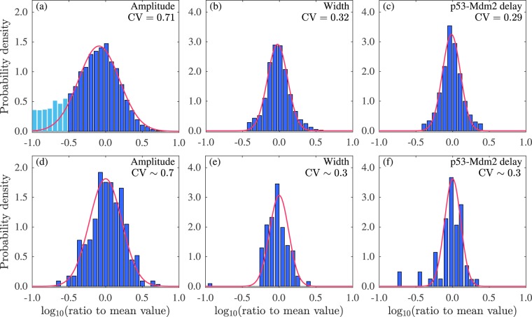
Figure 8.

Comparison of simulation results with the experimental data. The upper row shows the histograms for the base-10 logarithm of the peak amplitude and width of p53 oscillation and p53-Mdm2 delay divided by their respective mean values, respectively. The lower row shows the corresponding experimental data from ref.¹¹. 1000 runs of stochastic simulations lasting 3000 min are performed with S = 0.3, Ω = 10⁴, D = 0.04, and τ = 1000 min. Red curves are fittings by Gaussian density function (2πσ²)^−1/2exp[−(x − μ)²/(2σ²)] with (μ, σ) = (−0.091, 0.28) (a), (−0.026, 0.14) (b), (−0.017, 0.12) (c), (0, 0.22) (d), (0, 0.13) (e), and (0, 0.11) (f). The average CVs are marked in the figure. For (a)–(c), the CV can be estimated as follows: CV = σ₀/μ₀, where ${\mu }_0=\exp [(\mu +lo{g}_{10}\overline{x})\ln 10+{(\sigma \ln 10)}^2/2]$, ${\sigma }_0^2=\{\exp [{(\sigma \ln 10)}^2]-1\}\exp [2(\mu +lo{g}_{10}\overline{x})\ln 10+{(\sigma \ln 10)}^2]$, and $\overline{x}$ is the corresponding mean value: $\overline{x}=11761$ for amplitude, 118 min for width, and 101 min for p53-Mdm2 delay.