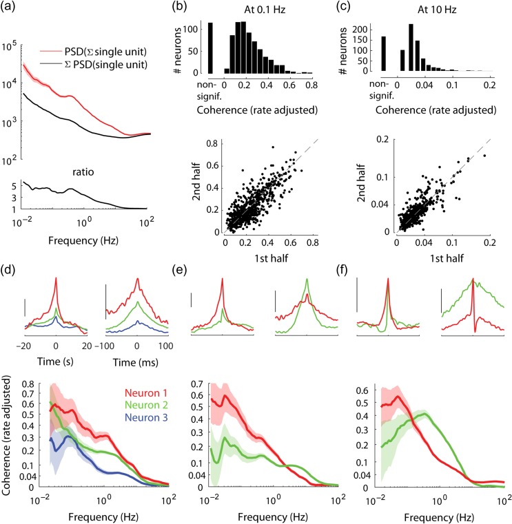
Figure 3.
Frequency-resolved population coupling. (a) Top: PSD of population rate and sum of PSDs of individual spike trains comprising the population rate, in an example recording. Bottom: the ratio between the two, indicating that in frequencies < 1 Hz the former is several-fold higher. (b) Top: Distribution of rate adjusted coherence with population rate at an example slow timescale frequency (0.1 Hz) across all neurons. Some neurons have no significant coherence (“non-signif.”). Bottom: rate adjusted coherence with population rate at 0.1 Hz, evaluated separately in first and second halves of the recordings, R2 = 0.63 (P < 10−100). (c) Same format as b, for fast time scale example frequency (10 Hz), R2 = 0.75 (P < 10−100). (d) Top: Time domain correlation between spike trains of 3 example simultaneously recorded neurons and the population rate, on slow and fast time scales (scale bar: median amplitude of the correlation across all neurons in the recording). Bottom: Rate adjusted coherence of each example neuron with population rate. (e) Two example simultaneously recorded neurons, where one (red) has high coherence with the population in low frequencies and low coherence in high frequencies, when compared with the other neuron (green), which exhibits the opposite behavior. Layout as in d. (f) Two example simultaneously recorded neurons whose relative strength of population coupling switches twice over the frequency range, furthermore one of the neurons (green) has a nonmonotonic coherence with population. Note that the time domain correlation with population rate of both neurons is of equal magnitude on both fast and slow timescales. Layout as in d. In c–f coherence values are shown using power function scaling, to make low values visible. In d–f shaded areas indicate 95% confidence intervals.

