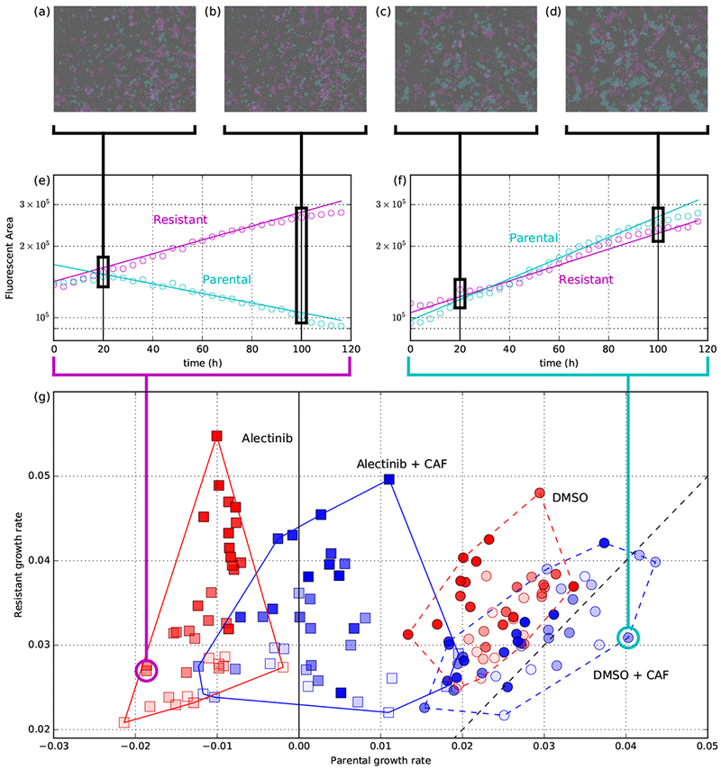
Figure 2: Coculture growth rates across four experimental conditions.

(a-f) serve as a sketch of the analysis procedure to produce the main subfigure (g); for more detailed discussion, see Supplementary Information Section B.4 (a,b,c,d): In each experimental replicate at each time step, we quantify population size by fluorescent area of each cell type (shown: two different time points per well, from two different wells). Together, 30 time-lapse microscopy images (one every 4 hours) from each replicate create (e,f): time-series of parental and resistant population size (shown: two example wells). With x-axis is time, y-axis is log of population size. Exponential growth rates (and confidence intervals; omitted) were estimated for each well using the Theil-Sen estimator. These exponential models are shown as solid lines and their slopes serve as the coordinates in (g). See Figure 3 for growth rate confidence intervals and Supplementary Information Section B.2 for detailed discussion of growth-rate measurement. (g): Each point is a separate replicate of a competitive fitness assay with initial proportion of parental cells represented by opacity and experimental condition represented by shape (DMSO: circle; Alectinib: square) and colour (no CAF: red; + CAF: blue). Each replicate’s x-position corresponds to the measured parental growth rate and y-position for resistant growth rate; the dotted black line corresponds to the line of equal fitness between the two at x = y.