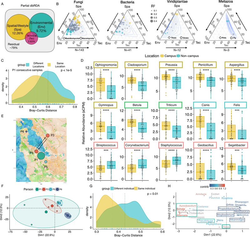
Fig. 3.

Decomposing the variation in the human environmental exposome. (A) Partial dbRDA variation partitioning analysis. (B) Ternary plots of variation partitioning analysis of highly prevalent genera (detected in >= 100 samples) in different domains of life. Environmental and spatial/lifestyle variables account for more than 80% of the explained variation in at least 75% genera. Each dot represents a genus and the size of the dot corresponds to the total explained variation. Depending on the genera, either environmental (blue) or spatial/lifestyle (dark yellow) variables may play dominant roles, or neither (grey). Contours denote 0.1 to 0.9 confidence intervals. (C) Samples from consecutive time points of P1 in the same location are more similar than those from different locations. (D) Representative differentially abundant genera between the “Campus” (N = 98) and non-”Campus” locations (N = 103). Boxes are color-coded as in Fig. 2A to denote the kingdom/subkingdom of the respective genus. (E) The location of the four individuals (P1, P3, P5, and P6) in the three-week parallel study. The size of dot corresponds to the self-reported activity level of each individual. Arrows indicate commute. (F) PCA analysis of P1, P3, P5 and P6. The bigger colored dots are geometric centers of respective groups. (G) Bray-Curtis distance profiles between samples from the same individual are more similar. (H) Top contributing genera with respect to the PCA analysis in (F). Color indicates relative contribution of each genus. All ellipses are drawn with axes equal to the standard deviation of the data. The Adj. p values are either directly displayed or denoted using the following notations * <0.05, ** < 0.01, *** < 0.001, and **** < 0.0001.