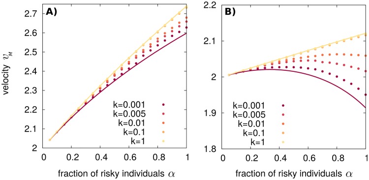
Fig 3. The asymptotic mean velocity increases with k in temporally varying environments.

(A) Velocities obtained by numerical integration of Eq 5 for s_a = 0.75, s_s = 1, s_b = 3 (yellow dot of Fig 2) for different switching rates k shown in the figure legend. (B) The same for s_a = 0.25, s_s = 1, s_b = 2 (blue dot of Fig 2). In (A), the optimal strategy is α = 1 for all k values. In (B), bet-hedging optimal strategies appear depending on the value of k. The continuous red and yellow lines (both in A and B) illustrate analytical predictions under the two limits v_M(k → 0) = (v_a(α) + v_b(α))/2 and $v_M(k\to \infty )=2\sqrt{D\langle \sigma \left(\alpha \right)\rangle }$, respectively.