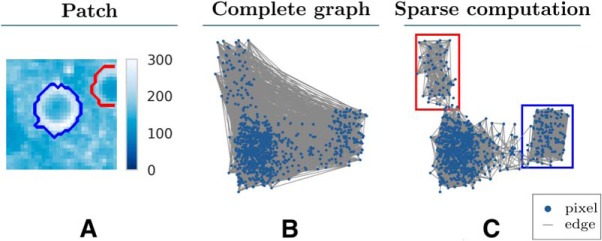
Figure 2.

Sparse computation constructs a sparse similarity graph. Comparison of a complete similarity graph and the similarity graph constructed by sparse computation for an example patch. For the purpose of illustration, the nodes are positioned based on the two-dimensional PCA projection of the feature vectors of pixels offset by a small uniformly sampled perturbation. A, Mean intensity image of the patch with the outline of two cells marked in red and blue. B, Complete similarity graph with an edge between every pair of pixels. For the purpose of illustration, only 10,000 randomly sampled edges are shown. C, Sparse similarity graph constructed by sparse computation with a three-dimensional PCA projection and a grid resolution of κ = 25. Two clusters of pixels (marked with red and blue rectangles) are identified by Sparse Computation. These two clusters match the spatial footprints of the two cells shown in A.