. 2019 Apr 12;8:e38619. doi: 10.7554/eLife.38619

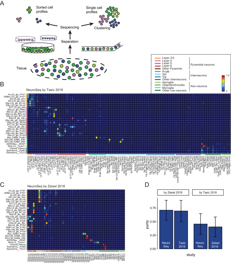
Figure 2. Decomposition by non-negative least squares (NNLS) fitting.

(A) Diagram illustrating potential sources of heterogeneity at the separation phase in profiles from sorted cells (left) or at the clustering phase in profiles from single cells (right). (B,C) NNLS coefficients of NeuroSeq cell populations decomposed by two scRNA-seq datasets: (Tasic et al., 2018; Zeisel et al., 2018). (D) Mean purity scores for NeuroSeq and SC datasets. The purity score for a sample is defined as the ratio of the highest coefficient to the sum of all coefficients. Error bars are Std. Dev.

Figure 2.

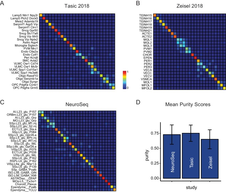
Figure 2—figure supplement 1. Self decompositions by NNLS.

Figure 2—figure supplement 1.

Each dataset is randomly divided into two groups and one is used to decompose the other. Coefficients matrix with perfect decomposition would be diagonal. Non-diagonal elements indicate limitation of the decomposition method due to having a subset of cell groups too similar to each other. (A–C) Heatmaps illustrate NNLS coefficients for subsets of samples in each dataset. Column order is same as row order. (A) 25 neocortical samples from Tasic et al. (2018), (B) 25 neocortical samples from Zeisel et al. (2018) and (C) 28 neocortical samples from present study. (D) Mean purity scores (as defined in Figure 2) for cross-validation (calculated over all neocortical samples) were comparable in each dataset. Error bars are Std. Dev.
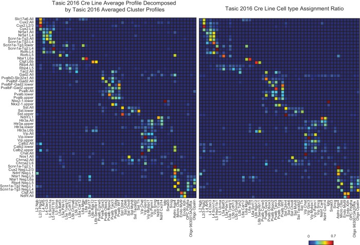
Figure 2—figure supplement 2. A validation of NNLS decomposition.

Figure 2—figure supplement 2.

(Left) Single-cell profiles from Tasic et al. (2016) were merged according to which of the 17 transgenic strains and sub-dissected layers they originated from (row labels). Merged profiles were then decomposed using individual cell type cluster profiles defined in Tasic et al. (2016) (column labels). (Right) The reported proportion of single-cell profiles according to the author’s classification. The close similarity between left and right matrices indicates an accurate NNLS decomposition of the merged clusters. Note that information about which and how many individual cell types were sorted from each line and set of layers was not explicitly provided to the decomposition algorithm, but were accurately deduced from the merged expression profiles.
Figure 2—figure supplement 3. NNLS decomposition of SC datasets: Tasic by Zeisel.
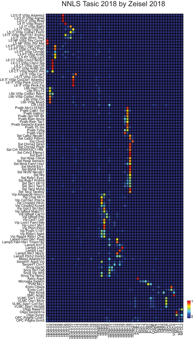
Figure 2—figure supplement 3.

The same neocortical samples from Tasic et al. (2018) and Zeisel et al. (2018) used in Figure 2 to decompose NeuroSeq neocortical samples were used to decompose each other. See Figure 2 for further details of cell identity. Order of samples listed is as in Figure 2. Presumably because Tasic et al. samples are more finely sub-clustered, individual Zeisel et al. samples (horizontal) frequently map to multiple Tasic samples (vertical).
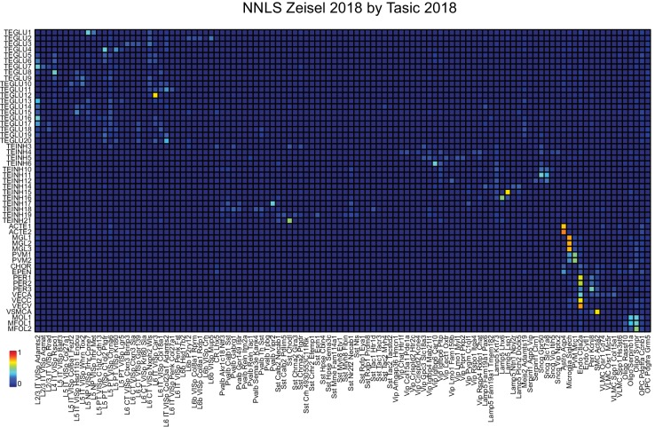
Figure 2—figure supplement 4. NNLS decomposition of SC datasets: Zeisel by Tasic.

Figure 2—figure supplement 4.

The same neocortical samples from Tasic et al. (2018) and Zeisel et al. (2018) used in Figure 2 to decompose NeuroSeq neocortical samples were used to decompose each other, but in the reverse order from the preceding supplementary figure. See Figure 2 for further details of cell identity. Order of samples listed is as in Figure 2.
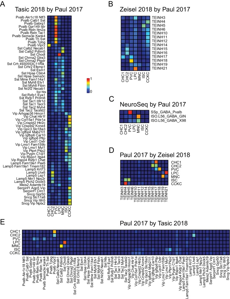
Figure 2—figure supplement 5. NNLS decomposition of interneuron datasets.

Figure 2—figure supplement 5.

Data from Paul et al. (2017), a third recent single-cell study focusing on neocortical interneurons, was used to decompose the cortical interneuron samples from (A) Tasic et al. (2018), (B) Zeisel et al. (2018), and (C) NeuroSeq. In addition, this data set was decomposed using the interneuron samples from the two other single cell data sets (D,E).
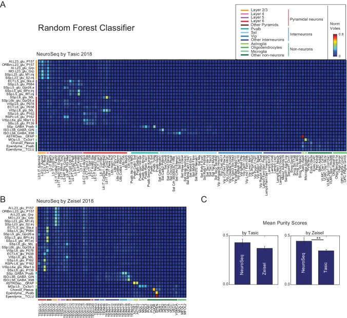
Figure 2—figure supplement 6. Random forest decomposition.

Figure 2—figure supplement 6.

A random forest classifier (500 decision trees) was trained from single-cell profiles (column labels) and then used to decompose NeuroSeq cell populations (row labels). Coefficients are the ratio of the votes from the 500 trees (coefficient ranges from 0 to 1 and 1 indicates all trees vote for a single class). The pattern of coefficients is similar to that obtained by NNLS (Figure 2) suggesting the decomposition is relatively robust and does not reflect a peculiarity of the NNLS algorithm.
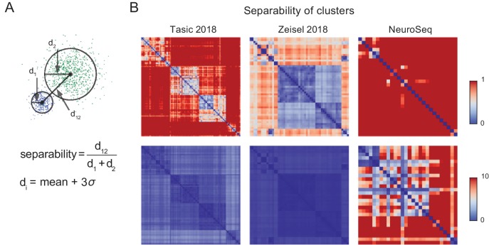
Figure 2—figure supplement 7. Separability of cell population clusters.

Figure 2—figure supplement 7.

(A) Definition of separability. Cartoon represents two different single-cell clusters as distributions of points. The separability is the ratio of the distance between the centroids to the sum of the 'diameter’ of each cluster. The diameter of a cluster is calculated as the mean distance to the centroid of the cluster +3 times the standard deviation of the distances of each point in the cluster. With this definition, two clusters are 'touching’ when separability =1, overlapping when <1, and separate when >1. The multi-dimensional distance is computed as 1- Pearson’s corr.coef. Note that averaging is expected to improve separability by roughly the square root of the number of cells averaged, hence most of the improved separability in the NeuroSeq data likely reflects averaging. (B) Separabilities between cell population clusters for three datasets shown with two different dynamic ranges (color scale; 0–1 for upper row and 0–10 for lower row). The order of cell population clusters are the same as in Figure 2.