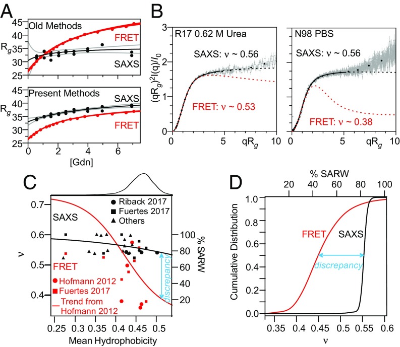
Fig. 1.
Improved analysis procedures do not eliminate discrepancy between SAXS- and FRET-derived measurements of IDP dimensions. (A) R17 SAXS and FRET data (from ref. 43). (A, Top) Comparison of results obtained when FRET data are fit assuming a Gaussian chain and SAXS data are fit using the Guinier approximation. (A, Bottom) SAXS and FRET data fit using our MFF analysis method and a similar approach (45). Black line is best fit hyperbolic trend line; gray lines are 95% confidence intervals. (B) SAXS profiles for R17 (Left, data from Ref. 43) and N98 (Right, data from ref. 42) fit with the MFF are significantly different from the expected behavior using values of ν taken from similar analysis of FRET data. Solid lines denote the region used in the fitting procedure; dashed lines represent extrapolation to higher values of q. Although ∼500 points per scattering curve were fit (gray), most data shown were binned for presentation purposes only (black points). The upturns or kinks in the data at higher values of qRg are most likely due to errors in buffer subtraction, which is more challenging at high q, low sample concentration, and/or reduced scattering contrast (e.g., at high denaturant, see Materials and Methods). (C) Trends of hydrophobicity (Kyte–Doolittle) versus ν in the absence of denaturant derived from SAXS by applying the MFF to published data collected from foldable protein sequences (42, 45, 67–82). Also shown are results from FRET studies calculated as in ref. 20 for published data (20, 42). Red trend line for FRET data from ref. 20. Black trend line is best fit to SAXS results shown. (C, Top) Histogram of hydrophobicity of representative proteins in the PDB (dataset from ref. 45). (D) Cumulative distributions of ν for the representative proteins from the PDB, inferred from the trend lines shown in C.

