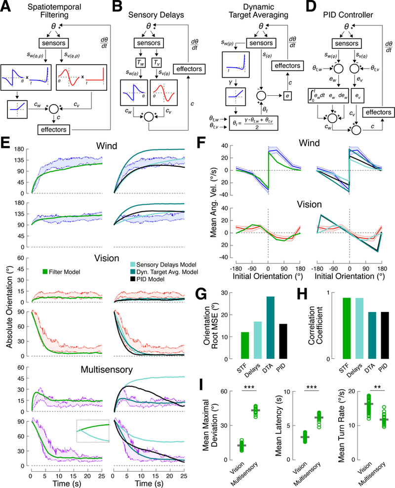
Figure 3. Summation of spatiotemporally filtered sensory inputs can account for turn slowing and turn sequences.

(A) Schematic of the spatiotemporal filtering model. Sensory signals for wind and vision, s_w(φ,ρ) and s_v(φ,ρ), are passed through spatial and temporal filters to generate turn commands, c, for each modality. Turn commands are summed and applied to heading, θ, generating new sensory signals on the next time step.

(B) Sensory delay model. Temporal filters are replaced by fixed processing delays (T) for each modality.

(C) Dynamic target averaging model. The turn command reflects the error, e, between current heading, θ, and target heading, θ_t. Target heading is a weighted average of target headings for vision (0°) and wind (180°). The time course of win d stimulation (s_w(ρ)) is temporally filtered to determine wind target weight.

(D) PID controller model. Sensory signals for each modality are compared to their respective target headings (0° for vision, 180° for wind) to g enerate an error for each modality. Turn commands are computed by summing proportional, integral, and derivative terms for this error. The overall turn command is a sum across modalities.

(E) Best fit simulations for each model compared to empirical data. Colored bands represent 95% confidence intervals for absolute orientation in response to wind (blue), vision (red), and multisensory (purple) conditions for flies starting at 0º and 90º. Left: spatiotemporal model (green, (A)). Right: delay model (light teal, (B)), dynamic target averaging model (dark teal, (C)), PID model (black, (D)). Note the differing y-axis scales. Best-fit parameters for each model are shown in Table 1. Inset shows the first 1 s of a simulation beginning at 60º for the spatiotemporal filtering and sensory delays models, highlighting the rapidity of the turning sequence generated by the latter. Inset vertical axis is 30º.

(F) Simulated turn rate as a function of orientation for each model compared to empirical data. Data (colored bands) is reproduced from Figure 1. Model colors as in (E).

(G) Root mean squared error between the best-fit simulation results, as shown in (E), and the empirical median absolute orientation time course. STF: spatiotemporal filtering model; Delays: sensory delays model; DTA: dynamic target averaging model; PID: PID controller model. Values shown in Table 1. The spatiotemporal filtering model fits the data best. See also Figure S6.

(H) Correlation coefficient between the empirical turn rate functions from (F) and the simulation results is plotted for each model. Correlation coefficient is used in place of RMSE to discount the effect of stimulus intensity. The models that do not include an explicit spatial filter do not fully capture the influence of orientation on turn rate.

(I) Measures of multisensory integration, computed for simulated behavior from the spatiotemporal filtering model. Each plot shows the simulated behavior of 20 “flies” (open circles). Each “fly” is the mean of 5 trials, mimicking the plots in Figure 2. Thick gray bars: mean across “flies.” All metrics are calculated as in Figure 2. Left: simulated flies turn farther from 0º in the multisensory condition compared to the vision condition (rank-sum test, p < 0.0001). Middle and right: simulated turns toward 0º in the multisensory condition occur later (p < 0.0001) and are slower (p < 0.01) than those in the vision condition.