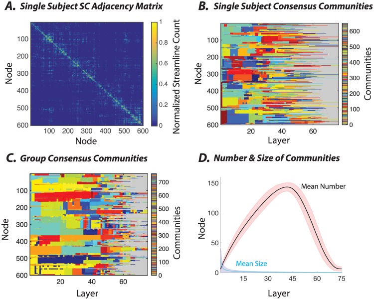
Fig 3. Application of multi-scale community detection to subject-level and group-level structural brain networks.

(A) An example structural connectivity matrix from one subject, in which each element linking a pair of brain regions represents the number of streamlines reconstructed between those two areas. To better visualize its structure, we apply a log transformation (log(SC + 1)/max(log(SC + 1))). (B) The consensus partition representing the multi-scale community structure for the matrix in panel (A). To enhance the visual detection of communities, we have represented all singleton communities with the same gray color. (C) The group-level consensus partition representing the multi-scale community structure for the structural matrix, which is defined as the consensus over all participants’ partitions. Here, again, to enhance visual clarity, we color the singleton communities in the same gray color. (D) The average number (out of 600 total nodes) as well as the average size (expressed as the percentage of total nodes) of the non-singleton communities calculated across layers, which in our case represent γ increments. In these analyses, we used γ ∈ [0.0133, 1], an inter-layer γ increment of 0.0133, and 75 layers.