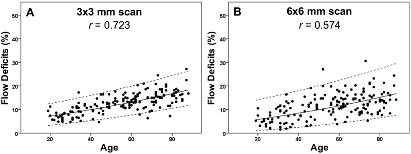
Figure 8: Adjusted scatter plots showing all the flow deficit percentages in the 2.5 mm circles with the 95% normal limits from the 3×3 mm scans and the 6×6 mm scans.
The solid line is the linear regression line after Y-axis back transformed from the square root of the flow deficit percentages. The dash lines represent the 95% normal limits. The correlation coefficient is r. (A) 3×3 mm scan. (B) 6×6 mm scan.

