. 2019 Apr 25;8:e43318. doi: 10.7554/eLife.43318

Figure 3. Individual-level behavioral quantification.

(A) Schematic explaining k-nearest neighbor density estimation. (B) Relative rate of reversals as a function of local density (k-nearest neighbor density estimation with k = 6) for npr-1 (blue) and N2 (orange) strains. Lines show means and shaded area shows the standard error (bootstrap estimate, 100 samples with replacement). (C) Distributions of crawling speeds at different local neighbor densities for both strains. Lines show histograms of speeds for each density bin, and the color of the line indicates the density (blue is high, magenta is low). (D) Midbody absolute speed for manually annotated npr-1 cluster entry (left, n = 28) and exit events (right, n = 29). Each event was manually identified, with time 0 representing the point where the head or tail of a worm starts to enter (left) or exit (right) an existing cluster. Skeleton xy-coordinates were linearly interpolated for missing frames for each event, before being used to calculate midbody speed extending 20 s on both sides of time 0 of the event. Speeds were smoothed over a one-second window. Shading represents standard deviation across events. Each red line shows the midbody absolute speed of a selected event that is shown in Video 3 (left) or Video 4 (right).

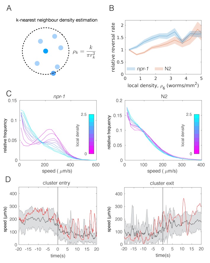
Figure 3.

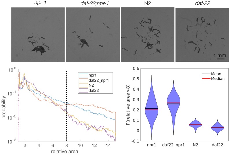
Figure 3—figure supplement 1. Pheromones appear unimportant for aggregation.

Figure 3—figure supplement 1.

npr-1 and N2 animals with pheromones removed by a daf-22 mutation aggregate to similar levels as their pheromone-intact counterparts. Top row: snapshots of 40 worms from each strain behaving on a thin, uniform lawn. Bottom left: quantification of cluster area relative to single worm area for each strain; dashed line shows the cut-off values used to generate the violin plot on the bottom right. Bottom right: probability of having a relative cluster area above the threshold value (dashed line on the bottom left). Blob area were extracted as tracking features. For each recording, a random sample (without replacement) of 500 single worms was used to calculate single-worm mean area, which was used to normalize multi-worm cluster areas from that recording. Relative cluster area values for each strain were pooled across recording replicates, and histograms were created with a bin width of 0.5.
Figure 3—figure supplement 2. Shape analysis for lone and in-cluster npr-1 worms.

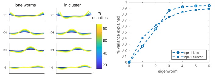
Figure 3—figure supplement 2.

Left two panels: first four eigenworms (Stephens et al., 2008) plotted in real space for projections of lone worms and in-cluster worms. Right: variance explained as a function of the number of eigenworms. Eigenworms are based on common reference (Brown et al., 2013) set for both strains and worm categories.