. 2019 Apr 25;8:e43318. doi: 10.7554/eLife.43318

Figure 6. Model with taxis captures quantitative aggregation phenotypes.

(A) Sample snapshot of the closest matching simulations for npr-1 (top) and N2 (bottom). (B) Summary statistics for npr-1 (orange) and N2 (blue): S1: pair correlation function; S2: hierarchical clustering distribution; S3: standard deviation of positions; S4: kurtosis of positions. Solid lines show the closest matching simulations; dashed lines show sample mean over the posterior distribution; and dotted lines show experimental means, with error bars showing standard deviation of 13 (npr-1) and 9 (N2) replicates. (C–D) Approximate posterior distribution of parameters for npr-1 (C) and N2 (D). Diagonal plots show marginal distribution of each parameter, off-diagonals show pairwise joint distributions. Parameters are: increase in reversal rate with density, r'; increase in rate to slow down, k's; decrease in rate to speed up, k'f; and contribution of taxis to motile force, ft.

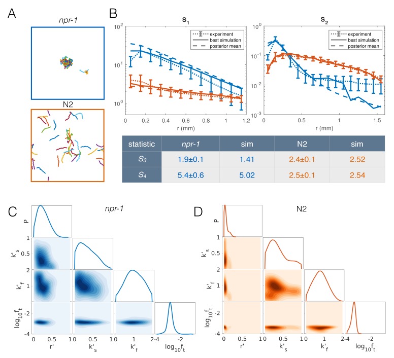
Figure 6.

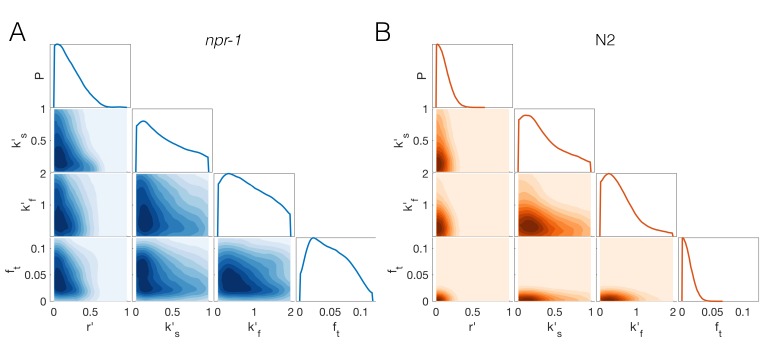
Figure 6—figure supplement 1. Reduced prior distribution used for approximate Bayesian inference of extended model.

Figure 6—figure supplement 1.

Marginal and joint prior parameter distributions for npr-1 (A) and N2 (B), that have been constructed from a set of pilot runs excluding any parameter combinations that lead to stable pairs for either strain, unstable clusters for npr-1, and stable clusters for N2. Remaining parameter values were used to construct the prior distributions via kernel-density estimation. See Appendix 1 for details.
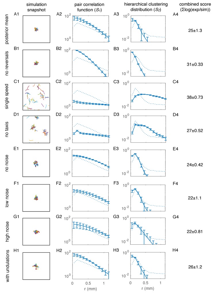
Figure 6—figure supplement 2. Core model components, but not noise and undulations in movement, are necessary for quantitative agreement with aggregation summary statistics.

Figure 6—figure supplement 2.

(A) Simulation for parameters equal to the mean of the posterior distribution for the npr-1 strain (Figure 6C). (A1), Sample snapshot of simulation; (A2), Pair correlation statistic, averaged over ten simulations (solid line), and standard error of the mean (error bars), with experimental reference (dotted line, as in Figure 6B); (A3), Hierarchical clustering distribution, averaged over ten simulations (solid line), and standard error of the mean (error bars), with experimental reference (dotted line, as in Figure 6B); (A4), Combined score for model agreement with experiment (lower score is better) for summary statistics in (A1) and (A2), calculated as the difference in the logarithm of the summary statistics between experiment and simulation (see Appendix 1 for details). (B) As in (A) but with r' = 0 (no reversals). (C) As in (A) but with worms always moving at the faster speed. (D) As in (A) but with ft = 0 (no taxis towards other worms). (E) As in (A) but with η = 0 (no directional noise in movement). (F) As in (A) but with η = 0.005. This η represents directional noise 10 times lower than in (A). (G) As in (A) but with η = 0.08. This η represents higher noise than in (A), and roughly corresponds to the velocity autocorrelation measured for interacting worms in our experiments (Figure 6 – figure supplement 4A2-3). (H) As in (A) but with sinusoidal undulations in the direction of movement, with a frequency similar to that of npr-1 worms (see Appendix 1 for details).
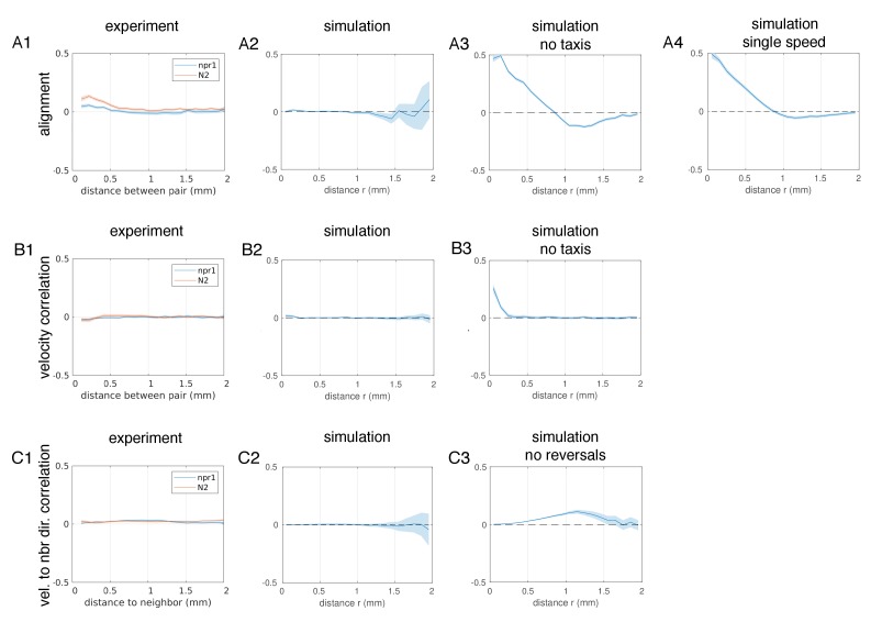
Figure 6—figure supplement 3. Analysis of orientational and velocity correlations in experiments and simulations.

Figure 6—figure supplement 3.

(A) Orientational correlation quantifies the alignment of the pharynxes (experiments, (A1), or first three nodes (simulations, A2-4) between pairs of worms a given distance apart. A value of 1 corresponds to parallel alignment, and −1 to anti-parallel alignment. Solid lines show the average directional correlation and shaded area shows the 95% confidence interval. (A1), Experimental measurements; (A2), Simulation for parameters equal to mean of posterior distribution for npr-1 strain (Figure 6C); (A3), As in (A2) but with ft = 0 (no taxis towards other worms); (A4), As in (A2) but with worms always moving at the faster speed. (B) Velocity correlation quantifies the alignment of movement directions between pairs of worms a given distance apart. A value of 1 corresponds to worms moving in the same direction, and −1 to worms moving in opposite directions. Solid lines show the average directional correlation and shaded area shows the 95% confidence interval. (B1), Experimental measurements; (B2), Simulation for parameters equal to the mean of the posterior distribution for the npr-1 strain (Figure 6C); (B3), As in (B2) but with ft = 0 (no taxis towards other worms). (C) Correlation between velocity of a worm and the direction to each neighbor was calculated to quantify the degree of taxis towards other worms. A value of 1 corresponds to worms moving directly towards a neighbor, and −1 to directly moving away from a neighbor. Solid lines show the average directional correlation and shaded area shows the 95% confidence interval. (C1), Experimental measurements; (C2), Simulation for parameters equal to the mean of the posterior distribution for npr-1 strain (Figure 6C); (C3), As in (C2) but with r' = 0 (no reversals).
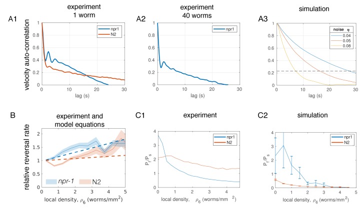
Figure 6—figure supplement 4. Additional comparison of model parameters with experimental measurements.

Figure 6—figure supplement 4.

(A) Velocity autocorrelation. (A1), From experiments with body wall muscle-tracked single worms on circular food patches; (A2), From experiments with 40 worms, of which a few were body wall muscle-tracked to allow acquisition of longer trajectories; (A3), From simulated, non-interacting worms undergoing a persistent random walk for different parameter values of η, the strength of the angular noise. The dashed line shows a value of 0.23, corresponding approximately to the expected correlation for choosing angles at random, uniformly distributed between −3/4π and 3/4π, thus representing an almost complete reorientation with respect to the original direction of motion. Note that this level is reached after about 15 s for η = 0.05 and for single worms (A1), and after about 8 s for η = 0.08 and interacting worms (A2). (B) Relative reversal rates at various local densities from experiments (solid lines and shaded 95% confidence interval, same data as in Figure 3B) and from model equations for reversal rates, parameterized with the mean of posterior distribution (dotted lines). (C) Speed switching rates at various local densities. (C1), Ratio of worms moving at fast (up to 350 μm/s) versus slow (<100 μm/s for npr-1,<50 μm/s for N2) speeds as measured in experiments; (C2), Ratio of worms moving at fast versus slow (<100 μm/s for npr-1,<50 μm/s for N2) speeds as measured in simulations with posterior mean parameters, showing average over ten (npr-1) and eight (N2) simulations, error bars showing error in the mean. The disagreement may indicate that the exponential form of kf(ρ) (see Figure 5C and main text) is only a rough estimate. For (B) and (CC), inferred model parameters were converted to units of worms/mm2.
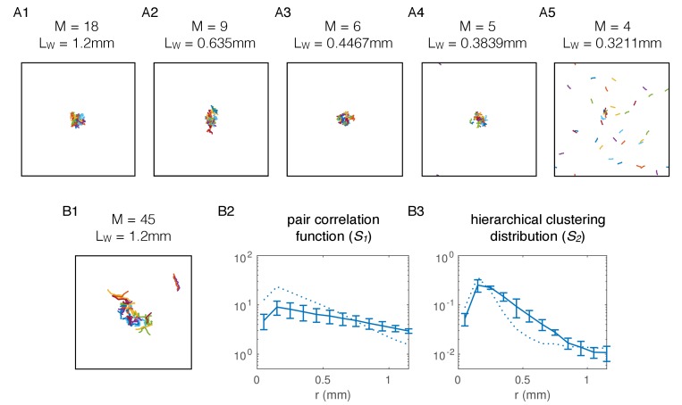
Figure 6—figure supplement 5. Aggregation model requires minimum length of simulated worms, and is robust to introducing volume exclusion.

Figure 6—figure supplement 5.

(A) Simulations with decreasing length of agents. (A1), Snapshot of simulation with posterior mean parameter values for npr-1, as in Figure 6—figure supplement 2A. Worms have M = 18 nodes and a total length of Lw = 1.2 mm; (A2), Modified model with M = 9 nodes and shorter worms (but same width) still produces aggregation, without readjusting other parameters; (A3), As in (A2) but with M = 6 nodes per worm and shorter total length; (A4), As in (A2) but with M = 5 nodes per worm and shorter total length; (A5), at M = 4 nodes per worm and corresponding length of Lw = 0.3211 mm, stable aggregates comprising all worms fail to form. At this worm length, the interaction radii of head and tail nodes start to overlap, and worms require a difference in contact between head and tail to initiate reversals in our simulations. (B) Simulations with volume exclusion. (B1), Snapshot of simulation where volume exclusion is enforced, such that worms cannot overlap (apart from themselves), without adjusting any other parameters. The number of nodes per worm has been increased to M = 45 to ensure sufficient overlap between nodes within a worm. Pair correlation function (B2) and hierarchical clustering distribution (B3) show that aggregate is spread out and less dense compared to experiments (dotted line). Solid lines show mean over three simulations and error bars show standard deviation.