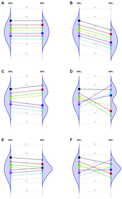
Figure 1. Scenarios representing fictional trials using 8 participants with systolic blood pressure as the primary endpoint.

Because of the random allocation to one of two treatment arms, we will observe only one of the two potential outcomes for each patient: either under T or under C. Fully saturated colors represent observed systolic blood pressure (SBP) values, and transparent squares represent missing potential SBP values. The line slope indicates the individual non-observable effect for each patient. Densities are the potential distributions of the outcome in each group: As both random samples come from the same target population, the average causal effect is estimable without bias. Panel A shows the potential outcome values that we could obtain if there were not any treatment effect; as the intervention has no effect at all, both groups have the same distribution (i.e., mean and variance). Panel B shows the scenario of a constant effect, meaning that the intervention lowers the SBP by a single value in every patient and thus implying the same variability in both arms. For instance, the study from Duran-Cantolla et al. ³ compared the 24-hour SBP in 340 patients randomized to either continuous positive airway pressure (CPAP) or sham–CPAP, and they observed a greater decrease of 2.1 mmHg (95% CI from 0.4 to 3.7) in the intervention group compared to the control group. Furthermore, baseline standard deviations (SDs) were 12 and 11; and final SDs were 13 for both groups. Therefore, their results fully agree with the trial design’s assumption of a constant effect (scenario B) and nothing contradicts the inference that each patient exhibits a constant reduction of 2.1mmHg, although uncertainty from sampling makes the results compatible with a constant effect that lies somewhere between 0.4 and 3.7. Panel C represents a situation with 2 different effects in 2 subpopulations (“treatment by subgroup interaction”). Although the effects are identical within them, the observable distribution in the treated arm would have higher variability. Here, finer eligibility criteria for classifying patients in those subpopulations might allow us to assume a constant effect again. In Panel D, the treatment has a variable effect in each patient, resulting also in greater variability within the treated arm but without any subgroup sharing a common effect. The results are poorly predictive about the effects on future patients. In the study by Kojima et al. ⁴, the primary outcome measure was the 3-hour postprandial area under the curve of apolipoprotein B48, with outcome SDs being, respectively, 0.78 and 0.16 in the treated and reference arms, thus showing an outcome variance ratio of 23.77. This is compatible with different treatment effects that could need additional refinements through precision medicine, since a greater variance in the treated arm indicates that “ the interpretation of the main treatment effect is controversial” ⁵. In that case, guidelines for treating new patients should be based either on additional eligibility criteria (“precision medicine”, panel C) or on n-of-1 trials (“individualized medicine”, panel D) ^{6– 10}. W. S. Gosset already highlighted this “treatment by patient interaction” in his 1908 paper, where he introduced the Student t-distribution ¹¹. Alternatively, interactions can result in smaller variances in the treated arm. Panel E shows a different effect in 2 subgroups; but the variability is now reduced, thus indicating that the best solution would be to identify the subpopulations in order to refine the selection criteria. In Panel F, the treatment again has a variable effect on each patient; but unlike Panel D, in this case the consequence is less variability within the treated arm. In the study from Kim et al. ¹², the primary endpoint was the PTSD Checklist–Civilian Version (PCL-C). This scale is based on the sum of 17 Likert-scale symptoms, ranging from 17 (perfect health) to 85 (worst clinical situation). At the end of the trial, the respective outcome SDs were 16 and 3 for the control and treated arms, meaning that variance was reduced around 28 times. This situation can correspond to scenarios E or F, and it merits statistical consideration, that is beyond the scope of this paper.