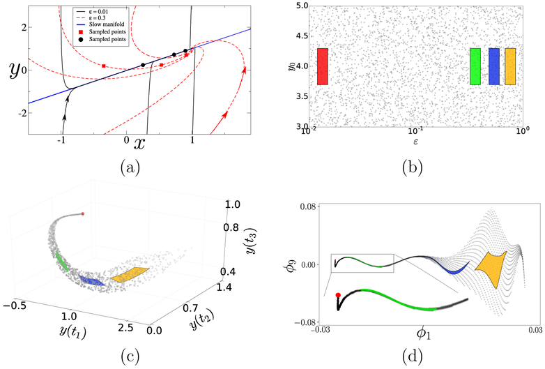
Figure 2:
(a) Phase portrait of (2) for a range of initial conditions (x0, y0) and two representative ε–values. Solid points mark states at the monitoring times (t1, t2, t3) = (0.5, 1, 1.5) for trajectories starting at x0 = −1. For ε = 0.01, the points lie close to the slow subspace and appear y0–independent; for ε = 0.3, instead, they lie off it and vary appreciably with y0. (b) A sample of the model input space, overlaid with distinct rectangular patches. (c) Mapping of the input sample of panel (b) to the 3–D output space. The images of the random sample outline part of the model manifold, while those of the patches show the dimensionality reduction due to the singularly perturbed structure of the model. (d) Mapping of the input sample in DMAPS coordinates. The transformations from (b) to (c–d) are discussed in the text.

