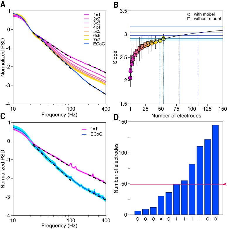
Figure 5.
PSD and slope analysis. A, Mean PSD across 77 LFP (pink; indicated as 1 × 1) and 5 ECoG (blue) electrodes and mean PSDs of signals obtained by first averaging the LFPs over progressively larger subgrids (pink to yellow). Slopes calculated for the 20–100 Hz and 200–400 Hz frequency ranges are plotted in dotted black (see Materials and Methods for details). The PSDs are normalized to have a value of 0 at 20 Hz for comparison of slopes. B, Average slopes and SDs (for 20–100 Hz frequency range) of the electrode grid combinations estimated with model (as described in Materials and Methods; circles) and without model (squares) are plotted on the y-axis (pink to yellow) for Monkey 3. The number of electrodes in each grid combination is plotted on the x-axis. Apart from squares as shown in A, we also considered rectangles of microelectrode populations (such as 2 × 3, 3 × 4, 4 × 6, etc.). The curve fitted on these slopes is shown in black. Blue horizontal lines are the experimentally determined slopes of the five ECoG electrodes for this monkey. The intersection of the fitted curve and ECoG slope yielded the number of LFP electrodes that needed to be averaged to produce the same slope as ECoG. C, Mean PSD of the LFP (pink) and ECoG (blue) averaged across four monkeys (Monkeys 1–4; data from Monkey 5 were not used because of the presence of noise at high frequencies). The SE is shown in lighter shade. Slopes are plotted in dotted black as before. D, Number of LFP electrodes that need to be averaged to match the slope of each of the 11 ECoG electrodes from four monkeys between 20 and 100 Hz (for Monkey 3, slope of one ECoG electrode was too steep and did not intersect the fitted black curve; see B). The symbols on the x-axis indicate the monkey (same as used in Fig. 4E). Red trace shows the median.

