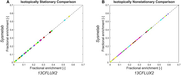
Figure 8.

Parity plots showing simulation results generated by 13CFLUX2 and Sysmetab. Classical, isotopically stationary approach (A) and INST ¹³C MFA approach (B). One color is used per measurement group. For comparability, both simulators were configured to use the same labeling framework, i.e., the reduced cumomers (Weitzel et al., 2007). Both simulators use sparse LU factorization for solving the cascaded cumomer systems. The differential equation systems were solved using Sundial's CVODE solver [https://computation.llnl.gov/projects/sundials/cvode/] (13CFLUX2) and a 4th order singly diagonally implicit Runge-Kutta method (Sysmetab). Both solvers used adaptive stepsize control with error tolerance (10⁻⁶). Simulation results and scripts for generating the parity plots are available in the Supplementary Data Sheet 2.