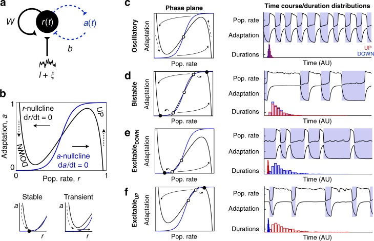
Fig. 2.
UP/DOWN dynamics in an adapting recurrent neural population. a Wilson–Cowan-like model for a neural population with slow adaptive process. b r-a Phase plane. Model dynamics are seen as trajectories in the phase plane that follow Equations (1–2). Dashed arrows indicate slow vertical trajectories at timescale of τa, solid arrows indicate fast horizontal trajectories at timescale of τr. Nullclines (the two curves along which dr/dt = 0, da/dt = 0) and their intersections graphically represent dynamics for a given set of parameter values (parameters as defined in C shown). Left and right branches of the r-nullcline correspond to DOWN and UP states, respectively. Stable UP/DOWN states are seen as stable fixed points at nullcline intersections. Transient UP/DOWN states are seen as r-nullcline branch with no intersection. c–f Four UP/DOWN regimes available to the model, as distinguished by location of stable fixed points (see also Supplementary Fig. 3). Representative phase plane (Left), simulated time course and UP/DOWN state duration distributions (right, time units arbitrary) for each regime. Stable fixed points are represented by filled circles, unstable fixed points by empty circles. Parameters: (c–f) b = 1, (c, e, f) w = 6 (d) w = 6.3, (c) I = 2.5 (d) I = 2.35 (e) I = 2.4 (f) I = 2.5. Default parameters specified in methods

