Figure 2.

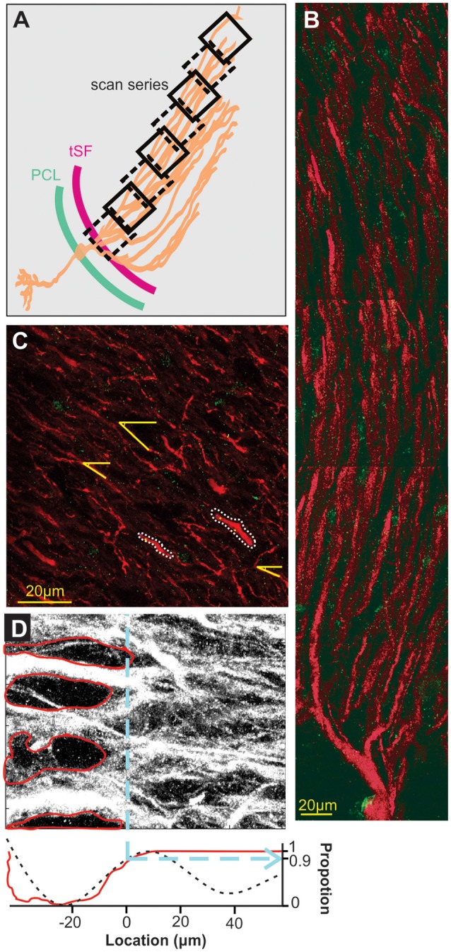
Scanning and localization procedure. (A) Scans arrangement. Each 105 × 105 μm scan is positioned relative to the transverse section of the ELL so that the first one of a series contains the tSF layer and subsequent ones overlap the previous and follow the orientation of dendrites in the molecular layer. Eight successive scans or more were performed to cover at least 600 μm of apical dendrites. (B) A series of scans showing the extensive apical dendritic bush in the molecular layer. Although we did not attempt to reconstruct and isolate single PC, our successive scans follow the apical dendrites of PCs. Red MAP2 labeling marks the inside of the dendrites and green labeling highlights the position of Nav channels. Since no distinction could be made between ON and OFF cells based on the immunolabeling used, all the dendrites quantified in the study are mixed, either ON or OFF-cells, and possibly VML interneurons (although it is unknown if they express dendritic Nav). (C) Dendrite selection and angle. Based solely on the MAP2 labeling (Nav labeling not displayed) we selected several clearly defined dendrites per scans for quantification (e.g., outlined with white dashes). Since dendrite orientation relative to the scan orientation is not orthogonal, we measured, in each scan, the average relative orientation of dendrites based on several dendrites per scan (yellow lines). This allowed us, using the position on the x-axis of the scan, the angle of dendrites and trigonometry, to determine a more accurate position of dendrites along the dendritic bush. (D) Determination of tSF dorsal edge to set it as location “0 μm”. The stratum fibrosum tract is characterized by large circular areas without MAP2 labeling between the large proximal apical dendrite shafts. We determined the dorsal edge of this layer by first highlighting the visible holes in labeling (red in the top image) and constructing a pixel histogram (red curve, bottom plot) along the x-axis based on the pixels outside these areas. Second, we used the raw pixel intensity values to build a histogram along the x-axis and smoothed it by fitting a triple sinusoid function (black dashes, bottom plot). Both histograms were normalized between 0 and 1 and we took the 0.9 mark of the rising slope to determine the 0 μm location (dashed blue line). We confirmed both histograms gave similar results and used the average of the two calculated values to set the 0-mark.