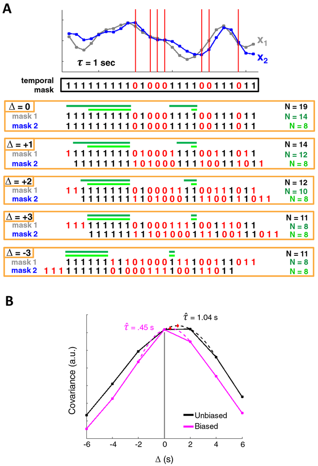
Figure 2. Cross-covariance among discontinuous time series.

(A) x₁ and x₂ are two surrogate time series. An example temporal mask shows censored time points in red (zeros). Although x₁ and x₂ share a temporal mask at zero-lag, computing cross-covariance requires that the time series be shifted with respect to one another, and with them, their associated temporal masks. Several shifts of the temporal masks are shown. To compute covariance at a given CCF lag, Δ, one could use all pairs of valid frames that align at that lag (all frames in black). This approach maximizes data usage but results in a substantially different number of samples (N) at each shift. Alternatively, one could restrict the minimum size of a block of non-censored data at zero-lag such that each block contributes at least one sample to every CCF lag (dark green). The minimum allowable block duration satisfying this requirement, is equal to the total number of lags (i.e.,Δ_max + 1 = 4 frames). This approach would limit (but not eliminate) uneven samples, at the cost of using less data. Note the symmetry of positive and negative CCF lags. Finally, a restriction may be imposed such that an equal number of samples contribute to each CCF lag, although this leads to still further data loss (light green). (B) CCFs for two surrogate time series, modeled at r = 0.9 and τ = 1 s, following censoring with a real temporal mask from a moderate-motion scan (MSC10 session 1). The black and pink CCFs represent the unbiased and biased CCF estimators, respectively. Note the triangular bias in the pink CCF, resulting in a τ value much lower than the true delay. Although the black CCF is quite accurate in this case, the unbiased estimator leads to $\widehat{\tau }$ values that have comparatively higher variance and may often exceed the true delay.