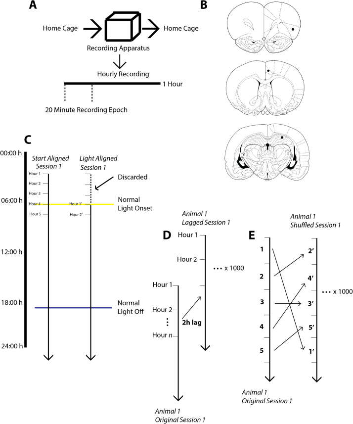
Fig. 1.

(A) The recording procedure for each of the long recording sessions. Animals are taken directly from their home cage and placed into the recording chamber where they remain for the next 60 h. In each of the 60 h, there is a 20 m epoch in which EEG data is acquired and the animal is encouraged to explore the environment through the random scattering of food pellets via the automatic pellet feeder. (B) Schematic coronal sections of rat brain illustrating the placement of electrodes in, from top to bottom, insular cortex, anterior cingulate cortex (ACC), and hippocampus. (C) Diagrammatic illustration of the light alignment procedure. In this example, a long recording session begins at 03:00. In the non-shifted start-aligned version, hour 1 of this recording session corresponds to 03:00. In the light-shifted version of this session, hour 1 is realigned to light onset and the four hours of recording that occurred before light onset are discarded. (D) Diagrammatic illustration of the data lagging procedure used to generate 95% confidence intervals in Fig. 2, Fig. 3. Lag magnitude varied between 0 and 58. Each dataseries was lagged 1,000 times individually. The lag magnitudes were drawn from a uniform distribution. This shuffling paradigm preserves the internal structure of each dataseries. (E) Diagrammatic illustration of the shuffling procedure used to generate the 95% confidence interval autocorrelation envelopes in Fig. 5, Fig. 6. Each of the 1–60 h is randomly reassigned to a new ordinal position in each of the 1000 shuffled dataseries. As in D), this shuffling procedure was performed 1,000 times on each of the dataseries.