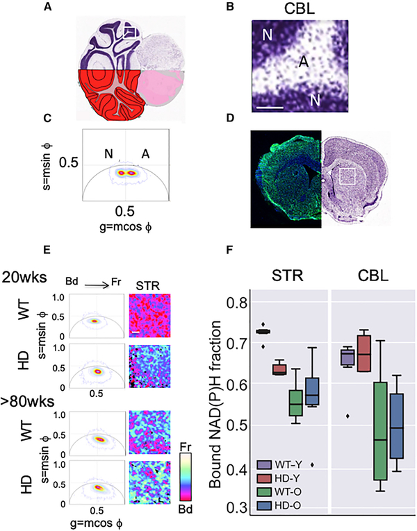
Figure 1. Abnormalities in Mitochondrial Metabolism Occur in Striatal MT in Living Brain Sections.

(A) Coronal section of a Nissl stained CBL illustrating dense neuronal-enriched layers in dark purple and astrocyte-enriched areas stained a diffuse purple. The segment shown in (B) is boxed in white.

(B) Magnified image of the boxed Nissl stained tissue section from (A). Scale bar is 100 μm.

(C) The two FLIM phasor distributions of NADH lifetimes (τϕ) for the neuron-rich (N) and astrocyterich (A) regions of the scanned CBL from HdhQ(150/150) (HD) mice have distinct average lifetimes. n = 3 tissue sections with two hundred scans per section, p values for all comparisons are indicated in (F). The phasors are calculated by transforming the lifetime decay data of each pixel in the imaged region to the phasor plot with co-ordinates (g = mcosϕ, s = msinϕ) where m is the modulation and ϕ is the phase shift of the fluorescence emission signal with respect to the excitation. The position of the phasor distribution indicates the free to bound NADH ratio with phasors on the right of g = 0.5 line having a higher free/bound ratio (or shorter lifetimes) than the ones in the left (longer lifetimes).

(D) Representative coronal section with prominent STR in a 15-week-old HdhQ(150/150) (HD) mouse brain. The left side is stained with NeuN antibody (neurons, green) and DAPI (all nuclei, blue). The right image is a Nissl stain. The white box indicates the scanned striatal region in the FLIM analysis in (E).

(E) Stacked FLIM phasor plots (left) from young (12- to 16-week-old) and old (>80-week-old) comparison of WT and HD mice, as in (C) for the CBL. Representative FLIM images for the STR, Scale bar, 100 mm. A pseudo-color scale for the free (Fr) and bound (Bd) fraction of NADH is shown.

(F) Box plot of the distribution of bound NADH fraction of CBL and STR of WT and HD animals at young (Y) (12–16 weeks) and old (O) ages (>80 weeks), as indicated. n = 3 tissue sections with two hundred scans per section. The box shows the quartiles of the bound NADH fraction dataset. The bars or whiskers extend to show the rest of the distribution, except outliers (shown as diamonds). The outliers are defined as points, which are more than 1.5 times the interquartile range above the third quartile or below the first quartile. p values, calculated by two-tailed Student’s t test. The p values for all comparisons in STR: HD-Y versus WT-Y (p = 7.7.× 3 10 ⁻⁷); HD-O versus WT-O (p = 0.84); HD-O versus HD-Y (p = 0.11); HD-O versus WT-Y (p = 0.0001); HD-Y versus WT-O (p = 0.005); and WT-O versus WT-Y (p = 4.1 × 3 10 ⁻⁶). The p values for all comparisons in the CBL: HD-Y versus WT-Y (p = 0.47); HD-O versus WT-O (p = 0.90); HD-O versus HD-Y (p = 0.007); HD-O versus WT-Y (p = 0.003); HD-Y versus WT-O (p = 0.03); and WT-O versus WT-Y (p = 0.02). See also Figure S1.