Figure - PMC

Skip to main content

An official website of the United States government

Here's how you know

Here's how you know

Official websites use .gov
A .gov website belongs to an official government organization in the United States.

Secure .gov websites use HTTPS
A lock ( ) or https:// means you've safely connected to the .gov website. Share sensitive information only on official, secure websites.

View full-text article in PMC

. 2018 Jan 13;39(4):1825–1838. doi: 10.1002/hbm.23971

Search in PMC
Search in PubMed
View in NLM Catalog
Add to search

© 2018 The Authors Human Brain Mapping Published by Wiley Periodicals, Inc.

This is an open access article under the terms of the http://creativecommons.org/licenses/by/4.0/ License, which permits use, distribution and reproduction in any medium, provided the original work is properly cited.

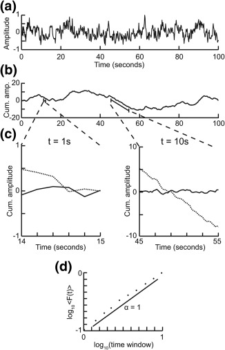
PMC Copyright notice

Step‐wise explanation of detrended fluctuation analysis. Adapted with permission from “Detrended fluctuation analysis: a scale‐free view on neuronal oscillations,” by R. Hardstone, S.S. Poil, G. Schiavone, R. Jansen, V. Nikulin, H.D. Mansvelder, and K. Linkenkaer‐Hansen, 2012, Frontiers in physiology, 3, 7. (a) Original time series. Taken from a 1/f signal sampled at 5 Hz with a duration of 100 s. (b) Cumulative sum of original signal shows large fluctuations away from the mean. (c) For each window size looked at, remove the linear trend from the signal, and then calculate the fluctuation. Signal shown as solid line and detrended signal shown as dotted line. (d) Plot the mean fluctuation per window size against window size on logarithmic axes. The DFA exponent is the slope of the best‐fit line (α = 1)