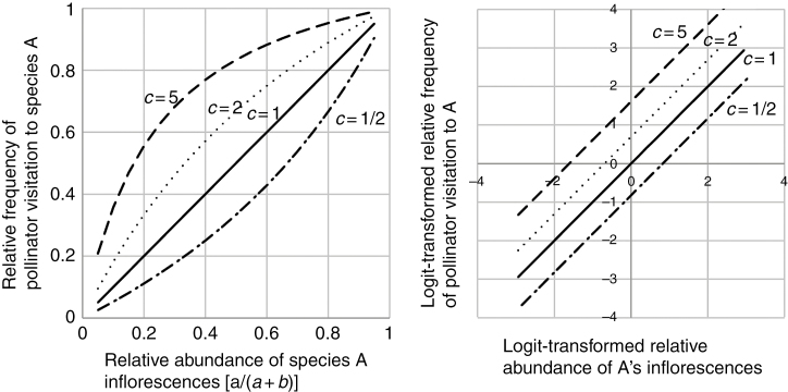
Fig 1.

Examples of regression curves (left graph) and logistic regression lines (right graph) calculated by using different values of pollinator preference c. When c = 1/2 (dash-dot lines), pollinators visited inflorescences of population B twice as many times as those of A, and when c = 1 (solid lines), pollinators showed no preference between inflorescence of populations A and B. When c = 2 (dotted lines), pollinators visited inflorescences of A twice as many times as those of B, and when c = 5 (dashed lines), they visited inflorescences of A five times more often than they visited those of B. The intercept of the logistic regression line is equal to the logarithm of c: log(1/2) = –0.693; log(1) = 0; log(2) = 0.693; and log(5) = 1.61.