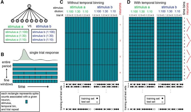
Figure 4.

Explanation of the basic classification procedure. A, All classifiers considered here discriminate among two different stimuli, each of which can be presented at one of three different dilutions. Thus, classifiers must overcome not only trial-to-trial variability, but also variability associated with stimulus intensity. Spheres at the bottom represent inputs for the classifiers. Each input corresponds to a given temporal window from a given neuron. For classifiers operating on a coarse timescale, the response of each neuron is represented by a single input. However, if responses are partitioned into multiple time bins, then each neuron contributes multiple inputs to the classifier. Thus, classifiers operating on finer temporal scales are associated with more inputs and weights. Lines represent classifier weights assigned during training. B, Response of a single neuron to a single stimulus presentation can be described in various temporal resolutions. In the top row, the entire postpresentation period is described as a single number (which is the average firing rate across the long window). Lower rows depict increasingly finer temporal resolutions. In these cases, individual trials are described as a sequence of firing rate values within smaller windows. C, D, Representation of the dataset without and with temporal binning. Each small rectangle represents spike counts associated with a particular neuron, stimulus, trial, and time period. The two rectangles represent data matrices associated with each of two stimuli. The difference between C and D is the extent of binning (a single time bin in C and five time bins in D). In both panels, the number of neurons shown is four. The circles at the bottom show examples of division of the dataset into training and test sets. One thousand such random divisions were made, and each was classified separately.