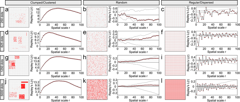
FIGURE 6.

Ripley’s L-function can detect three different point distribution patterns (clumped/clustered to the left-a, d, g, and j; random in the middle-b, e, h, and k; and regular/dispersed to the right-c, f, i, and l). Point patterns were generated with Matlab in a 100 × 100 square region. Each row shows the three distribution patterns generated with the same number of points: 250 in the top row, 625 in the second row, 1,250 in the third row, and 5,000 in the last row. In each subfigure, the left panel shows the actual point distribution and the right panel shows the corresponding L-function curve (the line with red data points) and the 95% confidence envelope for random distribution. The confidence envelopes in the clumped/clustered distributions with 1,250 and 5,000 points are very small thus they can hardly be seen on the L-function curve figures