Figure 5.

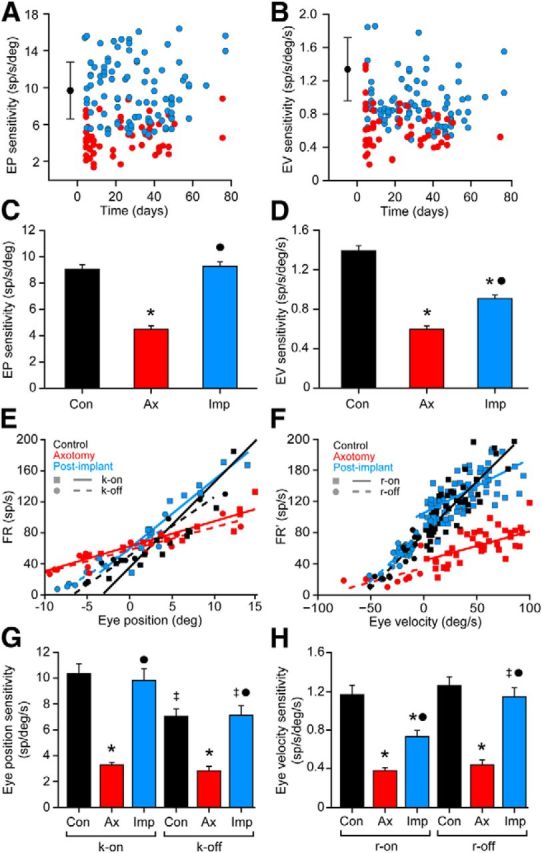
Analysis of the firing rate during spontaneous eye movements. A, Scatterplot of k values for axotomized (red) and postimplant (blue) abducens internuclear neurons represented versus time (days after the axotomy/implant). Control data are illustrated as a black dot (mean) with error bars (SD). B, Same as A, but for eye velocity sensitivity (r). C, D, Bar charts showing the mean ± SEM values of eye position sensitivity (k; C) and eye velocity sensitivity (r; D) obtained from neurons of the three experimental conditions: control (n = 68), axotomy (n = 57), and postimplant (n = 97). Significant differences with respect to control and axotomy groups are indicated by * and ●, respectively (p < 0.05; ANOVA test, Holm–Sidak method for multiple comparisons). E, Regression lines of FR versus eye position sorting those fixations attained after on-directed saccades (solid lines; k-on) from those after off-directed saccades (dashed lines; k-off) for an internuclear neuron of each group. F, Regression lines obtained after plotting the firing rate [minus the eye position component (FR′)] versus the eye velocity during on-directed (solid lines; r-on) or off-directed saccades (dashed lines; r-off) for an internuclear neuron of each group. G, H, Bar charts showing the on/off values (mean ± SEM) of eye position (G) and velocity (H) sensitivity, for 20 cells from each experimental population. Significant differences with respect to the control and axotomy groups for each parameter are shown by * and ●, respectively, while ‡ represents significant differences between the on and off parameters within the same group (p < 0.05; two-way ANOVA test, Holm–Sidak method for multiple comparisons).