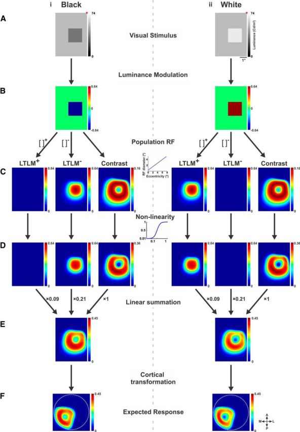
Figure 5.

Computing the expected response using a model. A, Visual stimuli. Left, Black stimulus. Right, White stimulus (lower left quadrants). B, Relative luminance values of each stimulus from A. Each pixel with respect to the luminance value present at the same location before stimulus onset (see Materials and Methods and Eq. 1). C, Values from B diverged into three pathways of processing: positive LTLM, negative LTLM (both obtained by rectification, Eqs. 5 and 6), and contrast (Eqs. 7 and 8). All three pathways are calculated using a weighted sum of a circular PRF (Eqs. 2 and 3) with a size that increases linearly as a function of eccentricity (Eq. 4). D, The three pathways from C, operated on by a nonlinearity function (Naka—Rushton; Eq. 9). Half-saturation values (C₅₀, L₅₀⁺, and L₅₀⁻) for the Naka–Rushton equation are calculated from response statistics in a surround field that is larger than the PRF, resulting in spatially specific divisive surround (Eqs. 10–12). E, The expected response obtained by linear summation of the three pathways from D (Eq. 13). F, The expected response after spatial transformation to cortical coordinates (V1) of the imaged eccentricities (see Materials and Methods for further details).