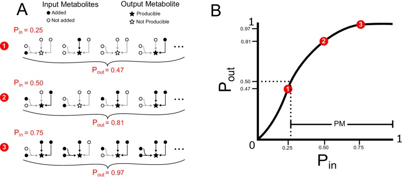
Figure 1. A probabilistic framework for calculating the producibility metric (PM).

(A) Random samples of input metabolites are added to the metabolic network with probability P_in. Samples are shown here with gray or red circles. Sampled input metabolites are then used to calculate if a specified target output metabolite can be produced or not. Here the solid red circled sample leads to production of the target metabolite while the dotted gray circled samples do not. The probability of producing the target output metabolite (P_out) is calculated by taking many random samples at a specified P_in. (B) A producibility curve is calculated which represents P_out as function of P_in. Points along this curve are sampled by assigning the P_in value and estimating P_out. The P_in value at which P_out = 0.5 (P_in,0.5) is used to define the producibility metric (PM) as PM = 1-P_in,0.5.

Figure 1—figure supplement 1. Probabilistic framework simple example.

(A) Input probabilities (P_in) are assigned to each input metabolite to designate the probability of adding that metabolite to the network. Random sets of input metabolites are sampled, based on P_in, and a modified version of flux balance analysis is used to determine if the network can produce a specified target output metabolite for each random sample. Many random samples are taken to estimate the output probability (P_out) of the target output metabolite. Three examples of P_in values and the corresponding P_out values are shown for a very simple network with three reactions, four input metabolites and one target metabolite. For this simple example, the output probabilities can be calculated using the probabilistic equation ${\displaystyle P_{out}=1-\left[{\left(1-P_{in}\right)}^2\ast \left(1-P_{in}^2\right)\right]=2P_{in}-2P_{in}^3+P_{in}^4}$. For more information on this theoretical calculation please refer to Figure 1—figure supplement 2. (B) A producibility curve is calculated which represents P_out as a function of P_in. Points along this curve are sampled by assigning the P_in value and estimating P_out. The three examples from A are shown in red on the curve in B. The PM is equal to one minus the value of P_in at which P_out equals 0.5 (P_in,0.5), such that increasing PM correspond to increasing producibility. In our implementation the PM for a particular metabolic network and metabolite is calculated efficiently using a non-linear fitting algorithm to find P_in,0.5. For further details on our exact implementation see the methods section “Algorithm functions: calc_PM_fit_nonlin.

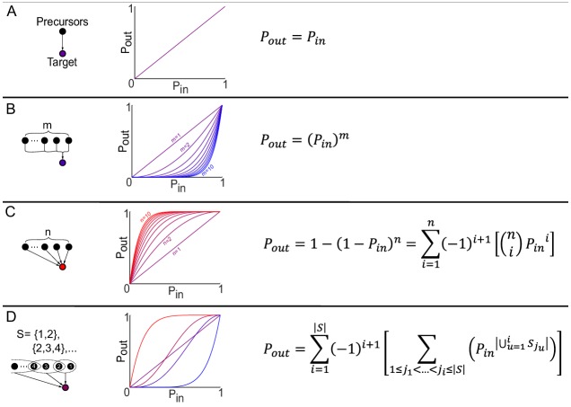
Figure 1—figure supplement 2. Theoretical properties of the producibility curve.

Theoretically, our method is closely related to the minimal precursor sets of a metabolic network. The minimal precursor sets describe all minimal subsets of metabolites that can be used to synthesize a particular metabolite or set of metabolites. A combinatorial formula was developed to calculate the value of P_out from the set of minimal precursor sets (S) and the value of P_in. Using this formula, an exact producibility curve can be plotted and theoretical values of the producibility metric (PM) can be calculated. This calculation is shown for increasingly complicated and general minimal precursor set structures. (A) In the simplest case, a single metabolite serves as the minimal precursor set for the target. This leads to a straight line producibility curve (P_out = P_in) and an expected PM value of 0.5. (B) If the target metabolite can be produced from one minimal precursor set of size m P_out is equal to P_in raised to the power of m due to the assumption that all metabolites are added independently. As m increases the producibility curve bows outward towards P_in = 1, and the PM decreases below 0.5. (C) If the target metabolite can be produced from n different minimal precursor sets of size 1 P_out can be defined based on the probabilistic rule for an or relationship, or it can be represented with a combinatorial formula. $\left(\begin{array}{c}n\\ i\end{array}\right)$ represents the binomial coefficients for n choose i. As n increases the producibility curve bows inward towards P_in = 0, and the PM increases above 0.5. (D) In the most general case, minimal precursor sets can be overlapping and any size/number. The producibility curve and PM vary depending on these properties. A combinatorial formula can be used to represent this general case. $\left|S\right|$ is the cardinality of the set of minimal precursor sets (the total number of minimal precursor sets). $\left|{\bigcup }_{u=1}^i{S}_{j_u}\right|$ is the cardinality of the union of the minimal precursor sets being enumerated by the recursive sum (the number of unique metabolites in the combination of minimal precursor sets being enumerated). The recursive sum over j_i enumerates all possible combinations of i minimal precursor sets by summing over the indices j_i where j_i is between j_i-1 and $\left|S\right|$, thus enumerating binomial combinations. The outer sum implements the inclusion exclusion principle.