Figure 2: Workflow for FCS-calibrated imaging.

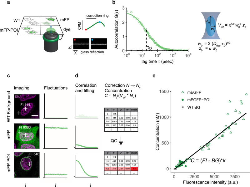
(a) Setup of the multi-well chamber with four different samples and optimization of the water objective correction for glass-thickness and sample mounting using a fluorescent dye and the reflection of the cover glass. dye: fluorescent dye to estimate the effective confocal volume, WT: WT cells, mFP: WT cells expressing the monomeric form of the FP, mFP-POI: cell expressing the fluorescently labeled POI.

(b) Computation of parameters of the effective confocal volume using a fluorescent dye with known diffusion coefficient D_dye and similar spectral properties as the fluorescent protein. Fitting of the ACF to a physical model of diffusion yields the diffusion time τ_D and structural parameter κ. The two parameters are used to compute the focal radius w₀ and the effective volume V_eff (Box 2).

(c) Images and photon counts fluctuations are acquired for cells that do not express a fluorescent protein (WT), cells expressing the mFP alone (mEGFP), and cells expressing the tagged version of the POI, mFP-POI (mEGFP-NUP107). The image fluorescence intensity (FI) at the point of the FCS measurement is recorded. Scale bar 10 μm.

(d) The ACF is fitted to a physical model to yield the number of molecules in the effective volume. WT concentrations are set to 0. After background and bleach correction concentrations are computed using the V_eff estimated in (a-b) and the Avogadro constant N_a.Data is quality controlled with respect to the quality of the fit and the amount of photobleaching using objective parameters.

(e) Concentrations estimated from FCS and image fluorescence intensities are plotted against each other to obtain a calibration curve (black line).