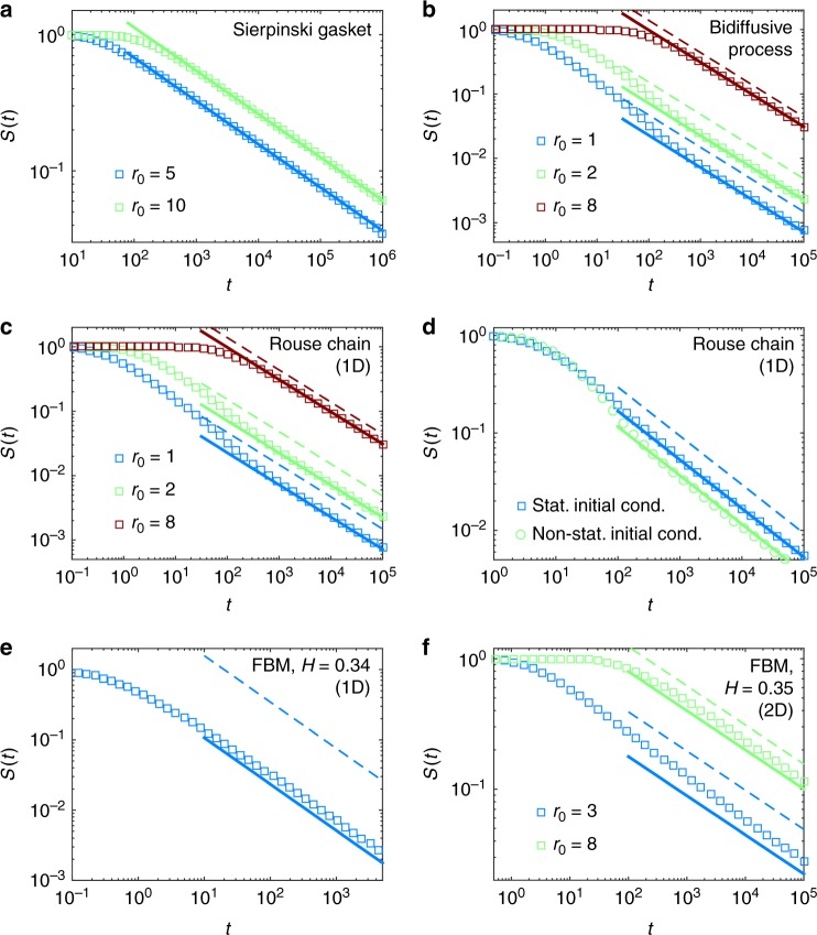
Fig. 2.

Survival probability $S\left(t\right)$ for various stochastic processes. In all graphs, symbols are the results of stochastic simulations (detailed in SI), continuous lines give the theoretical predictions (Eq. (18)), and dashed line represent the predictions of the pseudo-Markovian approximation (The pseudo-Markovian approximation, which is similar to the Wilemski–Fixman approximation for the polymer cyclization kinetics problem, consists in using effective propagators in Eq. (18), i.e $p\left(\mathbf{x},t\mid {\mathbf{x}}_0\right)=e^{-{\left(\mathbf{x}-{\mathbf{x}}_0\right)}^2∕2\psi \left(t\right)}∕{\left(2\pi \psi \left(t\right)\right)}^{d∕2}$.). a $S\left(t\right)$ for a random walk on the Sierpinski gasket for two values of the initial (chemical) source-target distance. Here, $d_f=\ln 3∕\ln 2$, $d_w=\ln 5∕\ln 2$, and $K\simeq 0.30$³¹. Simulations are shown for a fractal of generation $11$. Continuous lines are the predictions of Eq. (9). b $S\left(t\right)$ for a one-dimensional “bidiffusive” Gaussian process of MSD $\psi \left(t\right)=t+30\left(1-e^{-t}\right)$. c $S\left(t\right)$ for a one-dimensional Rouse chain with $N=20$ monomers, for various source-to-target distance $r_0$ (indicated in the legend in units of the monomer length). d $S\left(t\right)$ for the same system with $N=15$ and $r_0=3$, comparing stationary initial conditions (the other monomers being initially at equilibrium) or non-stationary ones (for which all monomers start at the same position $r_0$). e $S\left(t\right)$ for a one-dimensional FBM of MSD $\psi \left(t\right)=t^{2H}$ with Hurst exponent $H=0.34$. f Two-dimensional FBM of MSD $\psi \left(t\right)=t^{2H}$ in each spatial direction with $H=0.35$. The target is a disk of radius $a=1$ and $r_0$ is the distance to the target center. For (b), (c), (d), (e), and (f), the continuous lines represent our predictions (Eq. (18)), in which $\overline{T}$ is calculated by using the theories of refs. ^12,25,48; in (b) and (c) the only hypothesis to predict $\overline{T}$ is that the distribution of supplementary degrees of freedoms at the FPT is Gaussian, in (e) and (f) we use the additional “stationary covariance” approximation. In (d), for non-stationary initial conditions, $\overline{T}$ is measured in simulations in confined space. A table that compares the values of $S_0$ in the theory and in the simulations is given in SI