Fig. 2.

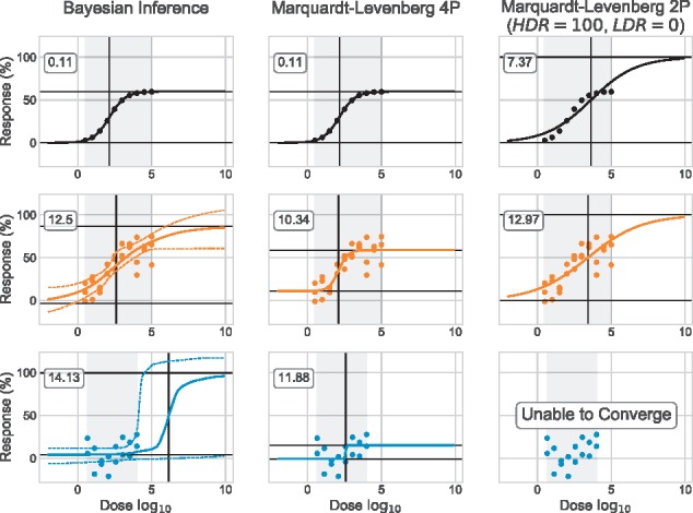
Marquardt–Levenberg versus Bayesian inference. Both synthetic datasets A₀ (black) and A₁₀ (orange) have triplicate (R = 3). The experimental dataset E₁ (blue) displays no response in the range of doses tested. Our Bayesian model is used to estimate dose–response curves with a 95% CI. Marquardt–Levenberg estimates the parameters of the 4P log-logistic model (Equation 1) and of the 2P model (only the IC₅₀ and S parameters are estimated: the HDR and LDR are fixed to constant values, 100 and 0, respectively). HDR and LDR (median values for Bayesian Inference) are represented by horizontal black segments; IC₅₀ (median value for Bayesian Inference). Root mean square error (RMSE) value is identified for each curve. For Bayesian Inference, we used the median curve to compute the residuals