Adversarial domain adaptation for cross data source macromolecule in situ structural classification in cellular electron cryo-tomograms

Abstract

Motivation

Since 2017, an increasing amount of attention has been paid to the supervised deep learning-based macromolecule in situ structural classification (i.e. subtomogram classification) in cellular electron cryo-tomography (CECT) due to the substantially higher scalability of deep learning. However, the success of such supervised approach relies heavily on the availability of large amounts of labeled training data. For CECT, creating valid training data from the same data source as prediction data is usually laborious and computationally intensive. It would be beneficial to have training data from a separate data source where the annotation is readily available or can be performed in a high-throughput fashion. However, the cross data source prediction is often biased due to the different image intensity distributions (a.k.a. domain shift).

Results

We adapt a deep learning-based adversarial domain adaptation (3D-ADA) method to timely address the domain shift problem in CECT data analysis. 3D-ADA first uses a source domain feature extractor to extract discriminative features from the training data as the input to a classifier. Then it adversarially trains a target domain feature extractor to reduce the distribution differences of the extracted features between training and prediction data. As a result, the same classifier can be directly applied to the prediction data. We tested 3D-ADA on both experimental and realistically simulated subtomogram datasets under different imaging conditions. 3D-ADA stably improved the cross data source prediction, as well as outperformed two popular domain adaptation methods. Furthermore, we demonstrate that 3D-ADA can improve cross data source recovery of novel macromolecular structures.

Availability and implementation

https://github.com/xulabs/projects

Supplementary information

Supplementary data are available at Bioinformatics online.

1 Introduction

Nearly every major process in a cell is orchestrated by the interplay of macromolecules, which often coordinate their actions as functional modules in biochemical pathways. Capturing the information on the native macromolecular structures and spatial organizations within single cells is necessary for the accurate interpretation of cellular processes. However, such information has been extremely difficult to acquire due to the lack of suitable techniques. Only recently, the advancement of the cellular electron cryo-tomography (CECT) 3D imaging technique has enabled the visualization of the sub-cellular structural organization in near-native state at sub-molecular resolution (Lučić et al., 2013). The advance of automatic image acquisition has made it possible for an electron microscope to capture hundreds of tomograms within several days, containing millions of structurally highly heterogeneous macromolecules (Oikonomou and Jensen, 2017). Each macromolecule is represented as a subtomogram, which is a cubic sub-volume enclosing the macromolecule extracted from a tomogram.

Due to the structural complexity of macromolecules and imaging limitations (missing wedge effects) in CECT data, the systematic macromolecule structural recovery is very challenging. Efficient and accurate structural classification of at least millions of highly heterogeneous macromolecules is a key step for such structural recovery. Since 2017, a number of convolutional neural networks (CNN)-based supervised subtomogram classification methods have been proposed (Che et al., 2018; Guo et al., 2018a; Xu et al., 2017). CNN has also been applied to other tomogram analysis tasks such as structural segmentation (Chen et al., 2017; Liu et al., 2018a, b), pattern mining (Zeng et al., 2018) and organelle detection (Li et al., 2019). Although deep learning-based subtomogram classification significantly outperformed existing high-throughput coarse classification methods in terms of speed and accuracy, they rely heavily on large amounts of properly labeled subtomograms.

In principle, it is feasible to label the training data through techniques such as template search (Beck et al., 2009; Kunz et al., 2015), unsupervised reference-free subtomogram classification (Bartesaghi et al., 2008; Chen et al., 2014; Xu et al., 2012), correlated super-resolution imaging (Chang et al., 2014; Johnson et al., 2015) or structural pattern mining (Xu et al., 2019). However, there are three main bottlenecks in the labeling process: (i) the aforementioned techniques are often computationally intensive, which may take weeks to complete, (ii) a substantial amount of manual quality control, including visual inspection and selection, is needed and (iii) most importantly, for each prediction dataset, a classification model needs to be trained using a valid training dataset from the same data source as the prediction dataset. Instead of preparing training data from the same data source, it would be beneficial to obtain training data from an independent data source preferably with labels readily available or can be prepared in an automatic and high-throughput fashion. Several independent data sources exist: (i) the electron cryo-tomograms of purified macromolecular complexes in which populations of macromolecules are already classified through biochemical means, (ii) simulated datasets, which provide an unlimited amount of data with fully automatic labeling and (iii) previously manually annotated datasets.

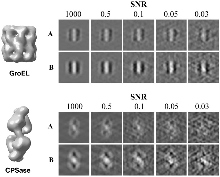
The main issue of using training data from an independent source is that it leads to a distribution difference between training data and prediction data. In other words, subtomograms containing the same structure but captured from separate data sources often have different image intensity distributions, which depends spatially on the relative 3D location on the macromolecular structure. For example, as in Figure 3, the same GroEL or CPSase under different imaging conditions appear differently. A classification model generally assumes the data distribution of training and prediction data to be identical (Tommasi et al., 2016). The differences between training and prediction data distributions can severely bias the model prediction. This phenomenon is termed domain shift, and is defined to be differences between training and prediction data in the joint distribution of input and output variables (Quionero-Candela et al., 2009).

Fig. 3.

Left: Isosurfaces of GroEL (PDB ID: 1KP8) and carbamoyl phosphate synthetase (PDB ID: 1BXR). Right: Center slices (x–z plane) of subtomograms from dataset batches A and B with different SNR levels

Formally, a domain$\mathbb{D}$ consists of two components, data (a dataset of subtomograms in our case) and a marginal probability distribution that the data follows, denoted as $\mathbb{P}(x)$. We refer to the dataset which labeled data are abundant as the source domain${\mathbb{D}}_s$, and the dataset which labeled data are not available or very little as the target domain${\mathbb{D}}_t$. For our CECT structural classification, the training subtomograms are sampled from the source domain and the prediction subtomograms are sampled from the target domain.

In this paper, we focus on a typical case of domain shift called covariate shift (Patel et al., 2015). Let x denote a subtomogram and y denote the class label of x. Covariate shift occurs in prediction problems when ${\mathbb{P}}_{x\sim {\mathbb{D}}_s}\left(y|x\right)={\mathbb{P}}_{x\sim {\mathbb{D}}_t}\left(y|x\right)$ but ${\mathbb{P}}_{x\sim {\mathbb{D}}_s}\left(x\right)\ne {\mathbb{P}}_{x\sim {\mathbb{D}}_t}\left(x\right)$. In other words, the conditional distribution of class labels y given subtomograms x is the same between source and target data, but the image intensity distributions between training and prediction subtomograms differ. This difference is primarily caused by different experimental conditions, such as resolution, defocus, spherical aberration and signal-to-noise ratio (SNR) (Fig. 3). Covariate shift has to be taken into account for cross data source classification.

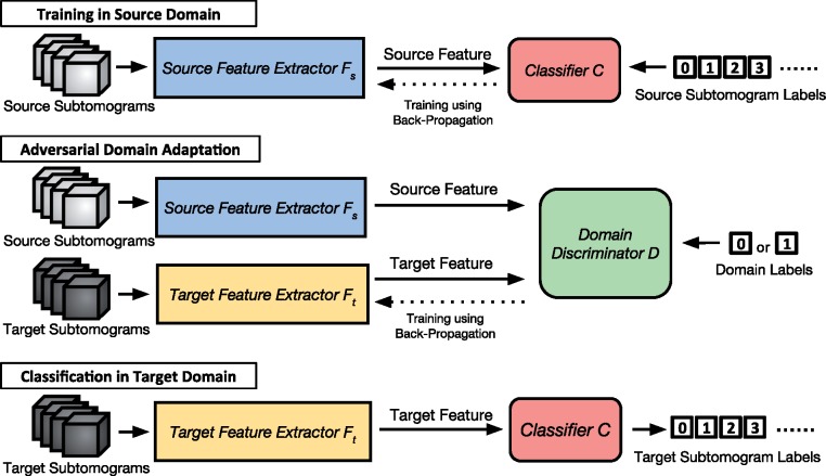
We adapt an adversarial learning approach for domain adaptation (from Ganin et al., 2016; Tzeng et al., 2017). The method is named adversarial domain adaptation (3D-ADA) and is shown in Figure 1. First, we train the combination of a source feature extractor $F_s$ and a subtomogram classifier C using labeled subtomograms from the source domain ${\mathbb{D}}_s$. Next, we train a target feature extractor $F_t$ and map the target domain features into a latent space with the similar distribution as the source domain features, using both labeled subtomograms sampled from the source domain ${\mathbb{D}}_s$ and unlabeled subtomograms sampled from the target domain ${\mathbb{D}}_t$. The mapping $F_t$ is learned using a domain discriminator D with an adversarial loss [Equations (1) and (2)], which minimizes the domain discrepancy. The training is conducted in an adversarial fashion: (i) the training of F_t aims to fool D so that D cannot discriminate features produced by F_t from features produced by F_s (Equation (1)), (ii) the training of D aims to maximally discriminate features produced by F_t from features produced by F_s (Equation (2)). This learning approach is inspired by the Generative Adversarial Network (GAN) (Goodfellow et al., 2014), which aims to confuse the discriminator D by generating images indistinguishable from the real ones. Different from GAN, 3D-ADA consists of feature extractors F_s and F_t, which are CNNs that map the input subtomograms into a low-dimensional feature space that are discriminative to the structural classes of the subtomograms. During the final classification, the trained target feature extractor F_t is used to extract features from subtomograms in the target domain ${\mathbb{D}}_t$, and input the discriminative features into the macromolecule structural classifier C to perform prediction.

Fig. 1.

An overview of the 3D-ADA framework. Those numbers in small white boxes are labels, including source subtomogram labels Y_s, target subtomogram labels Y_t and domain labels. Solid line arrays are inputs or outputs according to their directions. Dotted line arrays denote the training process here using the back-propagation algorithm

We tested 3D-ADA on 10 realistically simulated subtomogram datasets and three experimental datasets under different imaging conditions. 3D-ADA stably improved the cross-domain prediction, as well as outperformed two popular domain adaptation methods, Direct Importance Estimation (IE) (Sugiyama et al., 2008) and Structural Correspondence Learning (SC) (Blitzer et al., 2006). Furthermore, we demonstrate that 3D-ADA can also improve the cross data source structural recovery of novel macromolecules unseen in the training data.

2 Materials and methods

We have source domain subtomograms $X_s$ (i.e. 3D gray scale images of size $n\times n\times n$), represented as 3D arrays of ${\mathbb{R}}^{n\times n\times n}$. The source domain labels $Y_s$ are each represented as a binary array ${\{0,1\}}^l$, where l is the number of macromolecular structure classes in the source domain. We also have target domain subtomograms $X_t$ and their labels $Y_t$, in the same form as the source domain ones, respectively. Y_t is unknown and to be predicted after the domain adaptation.

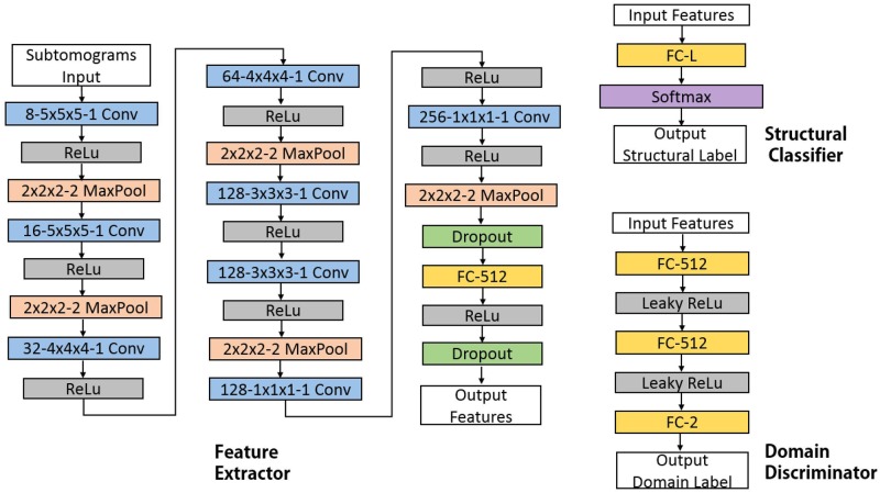
Source feature extractor F_s and classifier C are first trained using back-propagation on X_s and Y_s and using the standard cross-entropy as loss function. Next, we perform domain adaptation through adversarial training. Figure 1 shows our whole ADA method. The neural network models of F_s, F_t, C, D are illustrated in Figure 2. Specifically, we use the domain discriminator D, to classify the domain of the input data based on the extracted features. For D, the source domain label is set as 0 and target domain label is set as 1. F_t is initialized as a copy of the trained F_s. We then fix F_s and iteratively update F_t and D alternatively according to:

$$\begin{array}{cc}\hfill & \underset{F_t}{\min }{L}_F\left(D,X_s,X_t\right)=-{\mathbb{E}}_{x\hspace{0.17em}\sim X_t}\left(\text{log}\hspace{0.17em}\left(1-D\left(F_t(x)\right)\right)\right)\hfill \end{array}$$ (1)

$$\begin{array}{cc}\hfill & \underset{D}{\min }{L}_D\left(F_s,F_t,X_s,X_t\right)\hfill \\ \hfill & =-{\mathbb{E}}_{x\hspace{0.17em}\sim X_t}\left(\text{log}\hspace{0.17em}D\left(F_t(x)\right)\right)-{\mathbb{E}}_{x\hspace{0.17em}\sim X_s}\left(\text{log}\hspace{0.17em}\left(1-D\left(F_s(x)\right)\right)\right)\hfill \end{array}$$ (2)

Fig. 2.

Architectures of neural networks used in 3D-ADA. The networks include multiple layers which are represented by boxes in this figure and all of them are trainable. The type of layer and its critical parameters are shown in boxes. For example, ‘8−5×5×5−1 Conv’ denotes a 3D convolutional layer with eight 5×5×5 filters and stride of 1. It should be noted that ‘FC-L’ denotes a fully connected layer with L units, where L is the number of classes in datasets. These layers are defined similar to Zeng et al. (2018). Input and output of each module: for examples: input of F_s and F_t as subtomogram, input to C as features and output of C as structural classes, input to D as features, output of D as domains

D and F_t are trained in an adversarial fashion. Specifically, Equation (1) aims at training $F_t$ to trick the discriminator D. Clearly, $L_F$ will decrease when more target domain features are labeled close to 0 by D, so that it makes target domain features extracted by $F_t$ more possible to be regarded as source domain features by D. By contrast, Equation (2) aims at training a discriminative D to separate from target domain features from source domain features. $L_D$ will decrease when more source domain features are labeled close to 0 and more target domain features are labeled close to 1 by D. The ultimate goal of the adversarial training is to extract features invariant to domain change by the target feature extractor F_t. Ideally, in the ADA stage, the target feature extractor F_t should be trained to have the domain discriminator D has accuracy close to 0.5, meaning D is completely fooled by the domain invariant features extracted by F_t. 3D-ADA does not directly apply a min–max game in optimization as performed in the standard GANs (Goodfellow et al., 2014). The model is optimized by splitting a min–max loss into two independent losses, one for the F_t and one for D. The 3D-ADA method is shown in Algorithm 1.

After the ADA using Algorithm 1, the trained F_t is used to calculate ${\tilde{Y}}_t=C(F_t(X_t))$ for estimating Y_t, where ${\tilde{Y}}_t$ is predicted structure class labels Y_t of X_t. Because after domain adaptation, the distribution difference between $F_s(X_s)$ and $F_t(X_t)$ is reduced, C can be directly applied to $F_t(X_t)$ to calculate ${\tilde{Y}}_t$, with reduced biases from domain shift.

Algorithm 1.

Adversarial domain adaptation training

Input:

 Set of subtomograms from source domain: $X_s$

 Set of subtomograms from target domain: $X_t$

 Domain labels: $L_s=0$ and $L_t=1$

 Trained source feature extractor: $F_s$

Output:

 Trained domain discriminator: D

 Trained target feature extractor: $F_t$

 1:  forn training iterations do

 2:   fork steps do

 3:    Sample minibatch of m samples $\left\{x_s^1,\dots ,x_s^m\right\}$ from $X_s$.

 4:    Sample minibatch of m samples $\left\{x_t^1,\dots ,x_t^m\right\}$ from $X_t$.

 5:    Update D by ascending stochastic gradient of L_D, with F_t fixed:

$${▽}_{{\theta }_D}\frac{1}{m}\sum _{i=1}^m\left[-\text{log}\hspace{0.17em}\left(D\left(F_t\left(x_t^i\right)\right)-L_s\right)-\text{log}\hspace{0.17em}\left(L_t-D\left(F_s\left(x_s^i\right)\right)\right)\right]$$

 6:   Sample minibatch of m target samples $\left\{x_t^1,\dots ,x_t^m\right\}$ from $X_t$.

 7:   Update $F_t$ by descending stochastic gradient of L_F with the D fixed:

$${▽}_{{\theta }_{F_t}}\frac{1}{m}\sum _{i=1}^m\left[-\text{log}\hspace{0.17em}\left(L_t-D\left(F_t\left(x_t^i\right)\right)\right)\right]$$

 8:  returnD, $F_t$

The rationale behind using two training stages, one for extracting source features and the other for extracting target features invariant to domain change, is that we use the first stage to guarantee that features informative for classification is extracted. Intuitively, for subtomogram classification, if the two stages are trained simultaneously, the model could stuck in the local optimum that identical non-informative features are extracted to make the discriminator D completely fooled. However, such identical but non-informative features are useless for the classification in the target domain.

Compared to the original ADA method (Ganin et al., 2016), we have several modifications:

• We extended the 2D CNNs to 3D, and designed new 3D network architectures for CECT data.

• We use two feature extractors F_s and F_t to extract features from X_s and X_t separately [similar to Tzeng et al. (2017)] instead of a single one for both X_s and X_t. The independent $F_t$ for target data enables the target domain feature to be more flexible and robust.

• The adversarial loss function [Equations (1) and (2)] is gradient forwarded. The adversarial loss uses the proper domain supervision information for both D and $F_t$ training that avoids gradient vanish in back-propagation, thus the model is less likely to stuck in local minimum.

The details of the two baseline methods, Direct IE (Sugiyama et al., 2008) and SC (Blitzer et al., 2006), can be found in Supplementary Data.

3 Results

3.1 Simulated datasets

We generated two simulated dataset batches, denoted as dataset batch A and B (S_A and S_B). The two dataset batches differ in imaging parameters. Each batch contains five datasets of different SNR levels. Within each dataset, we simulated 23 000 subtomograms containing 23 structural classes.

The subtomogram datasets are realistically simulated by approximating the true CECT image reconstruction process similar to many previous works (Förster et al., 2008; Xu et al., 2012). Tomographic noise, missing wedges and electron optical factors, including the Contrast Transfer Function (CTF) and Modulation Transfer Function (MTF), were properly included, based on the assumption that macromolecular complexes have an electron optical density in proportion to the electrostatic potential. The PDB2VOL program from the Situs (Wriggers et al., 1999) package was used to generate subtomograms of 40³ voxels. The voxel spacing was defined to be 0.92 nm, the same as in experimental dataset $S_{e1}$ in Section 3.2 and the resolution was also defined at 0.92 nm. Electron micrographic images were simulated based on the density maps adopted from Protein Data Bank (PBD), through a tilt angle of $\pm {60}^{°}$. Noise was added to electron micrograph images (Förster et al., 2008) corresponding to different SNR levels, including the estimated SNRs from experimental data (Section 3.2). Optical effects were simulated by convolving the electron micrograph images the CTF and MTF (Frank, 2006; Nickell et al., 2005), with acquisition parameters similar to typical experimental tomograms (dataset $S_{e1}$ in Section 3.2).

Twenty-two representative macromolecular complexes (details in Supplementary Data) are collected from the PDB (Berman et al., 2000). Inside each dataset, for each complex, we generated 1000 simulated subtomograms, each containing a randomly rotated and translated macromolecule. Furthermore, we also simulated 1000 subtomograms that contain no macromolecule. As a result, one dataset contains 23 000 simulated subtomograms of 23 structural classes including the NULL class.

The two dataset batches each containing multiple datasets of different SNR levels (1000, 0.5, 0.1, 0.05, 0.03). The SNR of experimental datasets in Section 3.2 ranged from 0.01 to 0.5. Since we simulated 23 000 subtomograms within each SNR batch, in total there are 115 000 subtomograms in each batch. For S_A, we use the spherical aberration of 2 mm, defocus of −5 μm and voltage of 300 kV. For S_B, we use the spherical aberration of 2.2 mm, defocus of −10 μm and voltage of 300 kV. These parameters are assigned with typical values used in real CECT imaging (Xu et al., 2019; Zeev-Ben-Mordehai et al., 2016; Zeng et al., 2018). Dataset batch B has a higher contrast than dataset batch A because of its significantly higher defocus in magnitude. The MTF in our simulation is defined as $\mathrm{sinc}(\pi \omega /2)$ where ω is the fraction of the Nyquist frequency, a realistic detector (McMullan et al., 2009). To construct the final subtomogram, a direct Fourier inversion reconstruction algorithm [implemented in the EMAN2 library (Galaz-Montoya et al., 2015)] is used to produce the simulated subtomogram from the tilt series $\pm {60}^{°}$. Figure 3 shows examples of simulated subtomograms of two datasets batched with different SNRs.

3.1.1 Results on simulated data

We compared the macromolecule structural classification performance using dataset batch B (S_B) as training data and dataset batch A (S_A) as prediction data. Without domain adaptation, the prediction is calculated by $C(F_s(X_t))$. With domain adaptation, the prediction is calculated by $C(F_t(X_t))$ using F_t optimized using Algorithm 1.

The macromolecule structural classification accuracy is shown in Table 1. The accuracy is defined as the ratio of numbers of correctly classified samples to numbers of all samples. We also show the result of baseline methods IE and SC (details in Supplementary Data) performing the same tasks. In each cell, from top to bottom, the results displayed are accuracy without domain adaptation, IE accuracy, SC accuracy and 3D-ADA accuracy. The highest one is highlighted. The 3D-ADA framework achieved the highest accuracy in 24 of the 25 experiments. In addition, we discussed the impact of data augmentation on the prediction accuracy in Supplementary Data.

Table 1.

Accuracy on simulated datasets

Accuracy	SNR of target domain (SA)
		1000	0.5	0.1	0.05	0.03
SNR of source domain (SB)	1000	0.855	0.687	0.385	0.235	0.157
		0.739	0.620	0.287	0.159	0.111
		0.760	0.638	0.289	0.162	0.114
		0.991	0.923	0.737	0.499	0.326
	0.5	0.779	0.757	0.547	0.366	0.258
		0.806	0.710	0.479	0.372	0.291
		0.819	0.723	0.486	0.373	0.291
		0.978	0.970	0.835	0.628	0.464
	0.1	0.902	0.922	0.894	0.726	0.503
		0.864	0.881	0.776	0.637	0.475
		0.905	0.920	0.826	0.650	0.479
		0.894	0.932	0.901	0.760	0.626
	0.05	0.946	0.950	0.911	0.766	0.563
		0.937	0.929	0.897	0.758	0.575
		0.948	0.951	0.907	0.774	0.583
		0.967	0.971	0.928	0.825	0.628
	0.03	0.938	0.924	0.903	0.844	0.704
		0.903	0.891	0.864	0.775	0.609
		0.907	0.893	0.865	0.778	0.613
		0.976	0.972	0.952	0.891	0.773

Note: In each cell, from top to bottom, the results displayed are accuracy without domain adaptation, IE accuracy, SC accuracy and 3D-ADA accuracy. The highest one is highlighted in bold.

3.1.2 Result visualization

We visualize some of the results. Using subtomograms at SNR 0.1 in S_B as source and subtomograms at SNR 0.05 in S_A as the target, we randomly picked 100 samples in each target domain data class (2300 picked in total) to avoid crowdedness in the visualization. In Figure 4, we use T-SNE (Maaten and Hinton, 2008) to visualize their distribution before and after 3D-ADA. Figure 4 shows that, after 3D-ADA, structural classes become significantly more separable.

Fig. 4.

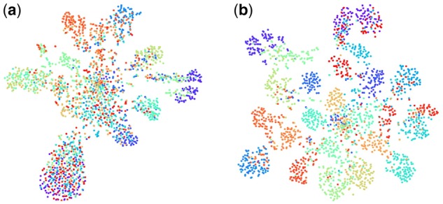
T-SNE embedding: target domain class prediction. Each dot represents a sample and its color represents its true class: (a) before 3D-ADA and (b) after 3D-ADA

The confusion matrices of the macromolecule structural classification results before and after 3D-ADA are shown in Figure 5. Clearly, after 3D-ADA, the misclassification rate is significantly reduced as the confusion matrix diagonal becomes darker after domain adaptation.

Fig. 5.

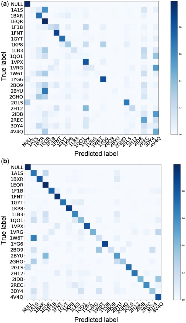
Confusion matrices of target domain class predictions: (a) before 3D-ADA and (b) after 3D-ADA. Each row represents the predicted class of an instance while each column represents the true class. The darker the cells are, the larger proportion of samples are predicted to be the specific class. A perfect classification will show a black diagonal with all cells on it having a value of 1.0

3.2 Experimental datasets

We further tested the 3D-ADA on three experimental datasets $S_{e1},\hspace{0.17em}{S}_{e2},\hspace{0.17em}{S}_{e3}$.

For $S_{e1}$, the experimental tomograms contain purified human 20S proteasome and Escherichia coli ribosome obtained through similar data generation procedure as in Zeev-Ben-Mordehai et al. (2016). To separate structures of trimeric conformations in native membrane-anchored full-length herpes simplex virus 1 glycoprotein B, imaging parameters have been successfully optimized and applied (Zeev-Ben-Mordehai et al., 2016). Specifically, Cryo-Electron Microscopy was performed at 300 keV using a TF30 ‘Polara’ electron microscope (FEI). The microscope was operated in zero-loss imaging mode with a 20-eV energy-selecting slit, using a Quantum postcolumn energy filter (Gatan). Images were recorded using a post-filter $\approx$4000 × 4000 K2-summit direct electron detector (Gatan). The detector was operated in counting mode with dose fractionation. A calibrated pixel size of 0.23 nm was adopted at the specimen level. Tilt series data were collected using SerialEM (Mastronarde, 2005) at defocus ranges of −6 to −5 μm. To have stable defocus during data collection, the auto-focusing routine was iterated through the tilt series with 100 nm accuracy. Finally, tomograms were reconstructed by the weighted back-projection in IMOD program (Sandberg et al., 2003). Then, the reconstructed tomograms were four times binned to result in a voxel spacing of 0.92 nm.

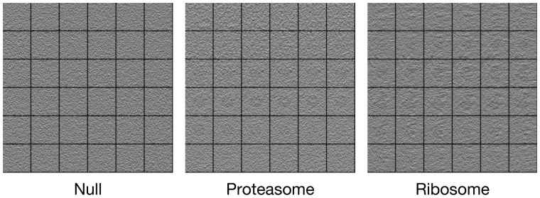
From three tomograms, we extracted a total of 4019 subtomograms of 36³ voxels. For each tomogram, we extracted subtomograms by performing template-free particle picking in a similar way to Pei et al. (2016). To extract the subtomograms, the tomograms were convolved with the 3D difference of a Gaussian, with scaling factor $\sigma =$5 nm and scaling factor ratio K = 1.1. The extracted subtomograms were smoothed by convolving with a Gaussian kernel of σ = 2 nm. We manually selected 100 ribosome subtomograms and 100 proteasomes, both with high confidence of their structure identity. In addition, we selected 100 subtomograms of NULL classes by randomly sampling the non-structural area of experimental tomograms. As shown in Figure 6, the experimental subtomograms has very low SNR (0.01) and thus highly challenging to classify. The templates were obtained from generating 4 nm resolution density maps from the PDB structures using the PDB2VOL program (Wriggers et al., 1999). Then, they were properly convolved with the CTF according to the imaging parameters. The templates are used to construct simulation datasets with labels as training datasets (source domain ${\mathbb{D}}_s$).

Fig. 6.

The 2D slices of example subtomogram in each class in dataset $S_{e1}$

Similarly, $S_{e2}$ contains 240 subtomograms, consisting of 80 ribosome subtomograms, 80 TRiC subtomograms and 80 proteasome subtomograms of size 40³ voxels with voxel spacing 1.368 nm. The subtomograms are manually extracted from a rat neuron tomogram (Guo et al., 2018b). The tilt angle range was $-{50}^{°}$ to $+{70}^{°}$. The structural templates were obtained using PDB structures 4GU0 (human 80s ribosome), 4V94 (eukaryotic chaperonin TRiC) and 6EPF (26S proteasome). The templates are used to construct simulation datasets with labels as training datasets (source domain ${\mathbb{D}}_s$).

$S_{e3}$ contains 400 hemagglutinin subtomograms, 400 apoferritin subtomograms and 400 insulin receptor subtomograms of size 28³ voxels with voxel spacing 0.94 nm from a single particle dataset (Noble et al., 2018). The tilt angle range was $-{60}^{°}$ to $+{60}^{°}$. The subtomograms are extracted using the difference of Gaussian particle-picking algorithm and manually annotated. The structural templates were obtained using PDB structures 3LZG (virus hemagglutinin), 4V1W (horse spleen apoferritin) and 4ZXB (human insulin receptor). The templates are used to construct simulation datasets with labels as training datasets (source domain ${\mathbb{D}}_s$).

3.3 3D-ADA classifications on experimental data

Based on different classes of macromolecules in different experimental dataset, we follow the simulation process mentioned in Section 3.2 to make their own source dataset.

For each training dataset, we simulated 3000 subtomograms for the source domain. The classification result is shown in Table 2. Since the classification of experimental subtomograms is very hard due to the high noise level and structural complexity, the classification accuracy before domain adaptation is virtually close to random guess (0.33). In all the experiments, 3D-ADA substantially increased the classification accuracy. How to choose the optimal simulation parameters to construct source dataset, especially structural templates and SNR, is still an open problem. Since when classifying an experimental subtomogram dataset, the data acquisition experimental conditions such as spherical aberration and defocus are known, we recommend the users to simulate training dataset with the same experimental condition parameters to reduce the domain shift between simulated source dataset and experimental target dataset. In terms of SNR, the simulated training dataset should have similar or slightly lower SNR as compared to the experimental dataset to be classified. However, the users should be aware that when the SNR of the training dataset is too low such as 0.001, the source dataset classifier training may not converge due to the strong influence of noise.

Table 2.

Accuracy of experimental subtomograms classification

Accuracy	SNR of source domain
Dataset	1000	0.5	0.1	0.05	0.03
$S_{e1}$	0.375	0.313	0.465	0.331	0.566
	0.578	0.641	0.563	0.584	0.606
$S_{e2}$	0.400	0.370	0.311	0.308	0.336
	0.495	0.469	0.471	0.450	0.377
$S_{e3}$	0.313	0.376	0.375	0.372	0.375
	0.688	0.656	0.625	0.621	0.624

Note: In each cell, the upper and lower numbers denote classification before and after 3D-ADA, respectively. The highest one is highlighted in bold.

We note here that in simulated dataset S_A and S_B, the number of subtomograms in the source domain and target domain is the same, 23 000. However, in practice, the number of subtomograms in the experimental datasets may be smaller. In our experiments on experimental data, there are 3000 subtomograms in the simulated source domain whereas the number of subtomograms in the experimental datasets varies from 240 to 300 to 1200. Although the number of subtomograms in the experimental target domain is significantly decreased, our 3D-ADA is still effective as shown in Table 2.

We applied a weighted subtomogram averaging algorithm (Xu et al., 2012) to recover the structure in $S_{e3}$ based on the classification label before and after domain adaptation (Fig. 7). The ground truth is obtained based on the true subtomogram labels. Although the apoferritin structure is successfully recovered even before using domain adaptation probably due to its strong signal and rotational symmetry, the hemagglutinin structure and the insulin receptor structure do not recover well using the classification label before the domain adaptation. By contrast, after 3D-ADA, we are able better recover the hemagglutinin structure and the insulin receptor structure. We note that the subtomogram number in $S_{e1}$ and $S_{e2}$ is too low to recover the structure.

Fig. 7.

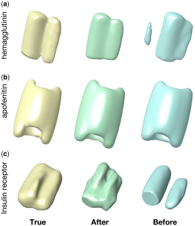
Recovered structures in S_e3 based on the classification label. Three structures: (a) Hemagglutinin, (b) Apoferritin, (c) Insulin receptor

3.4 Improvement of novel structure detection and recovery

Since the majority of macromolecular structures are still unknown, detecting novel structures in CECT is a key step to advance our in situ structural biology knowledge. Previously, we have demonstrated that even if prediction subtomograms contain unseen structural classes that do not exist in the training data, the unseen classes still tend to form clusters after being projected into the latent feature space using the trained feature extractor (Xu et al., 2017). Since the detection of novel structures depends on the extraction of important discriminative structural features, we investigate the novel structure detection when there is a covariate shift between source and target domains. We use subtomograms simulated at SNR 1000 in dataset batch B as X_s and subtomograms simulated at SNR 0.5 in dataset batch A as X_t. We removed all subtomograms of a particular structural class (RNA polymerase, PDB ID: 2GHO) from the training data. Denote the set of RNA polymerase subtomograms and their corresponding class labels in source and target domains as $X_s^{\text{RP}},\hspace{0.17em}{Y}_s^{\text{RP}},\hspace{0.17em}{X}_t^{\text{RP}}$ and $Y_t^{\text{RP}}$, respectively. We train F_s and C using $X_s\setminus X_s^{\text{RP}}$ and $Y_s\setminus Y_s^{\text{RP}}$, then obtain optimized F_t by applying the domain adaptation Algorithm 1 to $X_s\setminus X_s^{\text{RP}},\hspace{0.17em}{Y}_s\setminus Y_s^{\text{RP}}$ and $X_t\setminus X_t^{\text{RP}}$. Then we used T-SNE to further embed $F_s(X_t)$ and $F_t(X_t)$ into ${\mathbb{R}}^2$ to visualize the projected prediction samples before and after domain adaptation. Denote $F_{\mathrm{T}-\text{SNE}}$ as the T-SNE embedding. It can be seen from Figure 8 that the after domain adaption case, $F_{\mathrm{T}-\text{SNE}}(F_t(X_t^{\text{RP}}))$, is significantly better clustered than the before domain adaptation case, $F_{\mathrm{T}-\text{SNE}}(F_s(X_t^{\text{RP}}))$.

Fig. 8.

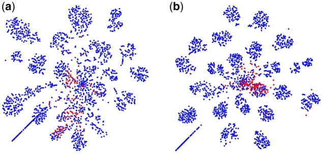
Subtomograms in the target domain projected to the structural feature space. The RNA polymerase (PDB ID: 2GHO) subtomograms which are removed from training process were highlighted in red: (a) before 3D-ADA and (b) after 3D-ADA

Moreover, we demonstrate for the cross-domain recovery of novel structures unseen in the training data. The extracted features are clustered into 100 clusters using k-means clustering. Then we applied a weighted subtomogram averaging algorithm (Xu et al., 2012) to recover the structure in each cluster. The recovered structures were manually matched to the 22 classes (including the novel one). To measure the structural discrepancy, we use the Fourier Shell Correlation (resolution) with 0.5 cutoff to show the maximal structural factors that are discrepant between the true structure and the recovered structure (Liao and Frank, 2010). Figure 9 shows examples of recovered structures and the novel structure RNA polymerase (2GHO) is successfully recovered with structural discrepancy 4.19 nm. To compare, the recovery of RNA polymerase before domain adaptation is 4.84 nm. Overall, the structural discrepancy of recovered structures before domain adaptation has mean value of 5.42 nm with a standard deviation of 1.28 nm. By contrast, the structural discrepancy after 3D-ADA has mean value improved to 5.17 nm with a standard deviation of 1.27 nm.

Fig. 9.

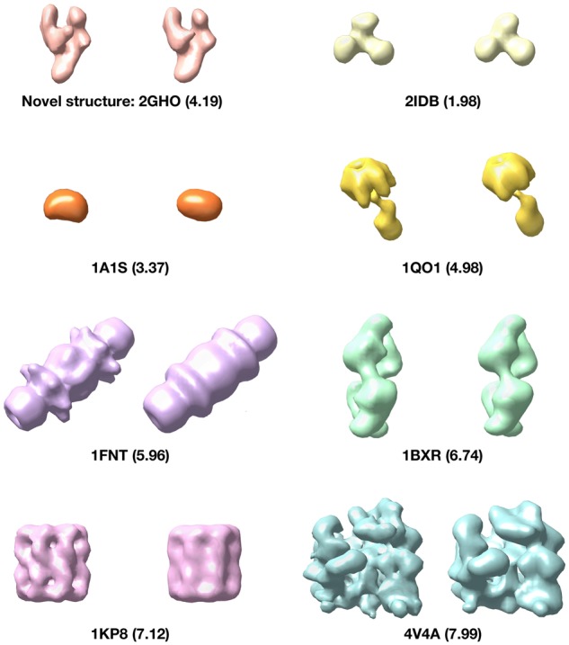
Structural recovery results. The underlying true structure is on the left and the recovered structure is on the right. The number in the parentheses denotes the structural discrepancy

4 Conclusion

Macromolecules are nano-machines that arguably govern cellular processes. In recent years, CECT has emerged as the most promising technique for the systematic and in situ detection of the native structure and spatial organization of macromolecules inside single cells. However, CECT analysis is very difficult due to the large data quantity, high level of structural complexity and imaging limitations in CECT data. High-throughput subtomogram classification is a key step in reducing structural complexity. Nevertheless, existing unsupervised subtomogram classification approaches either have limited accuracy or speed to process millions of structurally highly heterogeneous macromolecules available in a CECT dataset. Deep learning-based supervised subtomogram classification (e.g. Xu et al., 2017) potentially makes a powerful technique for the large-scale subtomogram classification with significantly improved speed and accuracy. But the successful training of such methods often require a large amount of structurally annotated subtomograms, which is generally laborious and computationally expensive to obtain from the same tomogram dataset. Therefore, it would be very beneficial to conduct the training using training data collected from a separate data source and annotated in a high-throughput fashion. In order to do so, the domain shift problem must be overcome as it is likely to significantly bias the results in the cross data source prediction setting.

We adapt an ADA framework for structural classification of macromolecules captured by CECT. Combining 3D CNNs and adversarial learning, 3D-ADA maps subtomograms into a latent space shareable between separate domains to obtain a robust model for cross data source macromolecular structural classification. Moreover, 3D-ADA can be easily extended to utilize multiple CECT training data sources by training multiple source domain feature extractors.

Most traditional domain adaptation methods aim to minimize some metric of domain shift such as maximum mean discrepancy or correlation distances. Other methods try to reconstruct the target domain from the source representation. Compared with those traditional methods, the ADA has the following advantages for CECT data:

• Using deep learning techniques, 3D-ADA allows large-scale training with large amounts of prediction data.

• Instead of using fixed features, the feature extractor is trainable and the domain adaptation is incorporated into the training process. The final classification is performed on adapted features that tend to be discriminative with respect to structural classes and invariant with respect to domains.

• Using the back-propagation algorithm, 3D-ADA is constructed as end-to-end feed-forward networks, improving over the isolated domain adaptation steps.

Our tests showed that our 3D-ADA significantly improved cross data source subtomogram classification, and it outperformed two classical domain adaptation methods. 3D-ADA can also potentially be useful for cross data source detection novel macromolecular structures.

This work represents an important step towards fully utilizing the power of deep learning for large-scale subtomogram classification. The optimal CNN models and training strategies for more accurate domain adaptation remain to be explored.

References

- Bartesaghi A. et al. (2008) Classification and 3D averaging with missing wedge correction in biological electron tomography. J. Struct. Biol., 162, 436–450. [DOI] [PMC free article] [PubMed] [Google Scholar]
- Beck M. et al. (2009) Visual proteomics of the human pathogen Leptospira interrogans. Nat. Methods, 6, 817–823. [DOI] [PMC free article] [PubMed] [Google Scholar]
- Berman H. et al. (2000) The protein data bank. Nucleic Acids Res., 28, 235.. [DOI] [PMC free article] [PubMed] [Google Scholar]
- Blitzer J. et al. (2006) Domain adaptation with structural correspondence learning. In: Proceedings of the 2006 Conference on Empirical Methods in Natural Language Processing, pp. 120–128. Association for Computational Linguistics, Sydney, Australia.
- Chang Y.-W. et al. (2014) Correlated cryogenic photoactivated localization microscopy and cryo-electron tomography. Nat. Methods, 11, 737–739. [DOI] [PMC free article] [PubMed] [Google Scholar]
- Che C. et al. (2018) Improved deep learning-based macromolecules structure classification from electron cryo-tomograms. Mach. Vision Appl., 29, 1227–1236. [DOI] [PMC free article] [PubMed] [Google Scholar]
- Chen M. et al. (2017) Convolutional neural networks for automated annotation of cellular cryo-electron tomograms. Nat. Methods, 14, 983.. [DOI] [PMC free article] [PubMed] [Google Scholar]
- Chen Y. et al. (2014) Autofocused 3D classification of cryoelectron subtomograms. Structure, 22, 1528–1537. [DOI] [PubMed] [Google Scholar]
- Förster F. et al. (2008) Classification of cryo-electron sub-tomograms using constrained correlation. J. Struct. Biol., 161, 276–286. [DOI] [PubMed] [Google Scholar]
- Frank J. (2006) Three-Dimensional Electron Microscopy of Macromolecular Assemblies. Oxford University Press, New York. [Google Scholar]
- Galaz-Montoya J.G. et al. (2015) Single particle tomography in eman2. J. Struct. Biol., 190, 279–290. [DOI] [PMC free article] [PubMed] [Google Scholar]
- Ganin Y. et al. (2016) Domain-adversarial training of neural networks. J. Mach. Learn. Res., 17, 2096–2030. [Google Scholar]
- Goodfellow I. et al. (2014) Generative adversarial nets In: Advances in Neural Information Processing Systems 27: Annual Conference on Neural Information Processing Systems 2014, December 8–13, 2014. Montreal, Quebec, Canada, pp. 2672–2680. [Google Scholar]
- Guo J. et al. (2018a) Model compression for faster structural separation of macromolecules captured by cellular electron cryo-tomography. In International Conference Image Analysis and Recognition, pp. 144–152. Springer, Póvoa de Varzim, Portugal. [DOI] [PMC free article] [PubMed]
- Guo Q. et al. (2018b) In situ structure of neuronal c9orf72 Poly-Ga aggregates reveals proteasome recruitment. Cell, 172, 696–705. [DOI] [PMC free article] [PubMed] [Google Scholar]
- Johnson E. et al. (2015) Correlative in-resin super-resolution and electron microscopy using standard fluorescent proteins. Sci. Rep., 5, 9583. [DOI] [PMC free article] [PubMed] [Google Scholar]
- Kunz M. et al. (2015) M-free: mask-independent scoring of the reference bias. J. Struct. Biol., 192, 307–311. [DOI] [PubMed] [Google Scholar]
- Li R. et al. (2019) Automatic localization and identification of mitochondria in cellular electron cryo-tomography using faster-RCNN. BMC bioinformatics, 20, 132. [DOI] [PMC free article] [PubMed] [Google Scholar]
- Liao H.Y., Frank J. (2010) Definition and estimation of resolution in single-particle reconstructions. Structure, 18, 768–775. [DOI] [PMC free article] [PubMed] [Google Scholar]
- Liu C. et al. (2018a) Deep learning based supervised semantic segmentation of electron cryo-subtomograms. In IEEE International Conference on Image Processing, pp. 1578–1582, ICIP, Athens, Greece. [DOI] [PMC free article] [PubMed]
- Liu C. et al. (2018b) Multi-task learning for macromolecule classification, segmentation and coarse structural recovery in cryo-tomography. In: British Machine Vision Conference, BMVC, p. 271, North Umbria University, Newcastle, UK. [PMC free article] [PubMed]
- Lučić V. et al. (2013) Cryo-electron tomography: the challenge of doing structural biology in situ. J. Cell Biol., 202, 407–419. [DOI] [PMC free article] [PubMed] [Google Scholar]
- Maaten L.V.D., Hinton G. (2008) Visualizing data using T-SNE. J. Mach. Learn. Res., 9, 2579–2605. [Google Scholar]
- Mastronarde D.N. (2005) Automated electron microscope tomography using robust prediction of specimen movements. J. Struct. Biol., 152, 36–51. [DOI] [PubMed] [Google Scholar]
- McMullan G. et al. (2009) Detective quantum efficiency of electron area detectors in electron microscopy. Ultramicroscopy, 109, 1126–1143. [DOI] [PMC free article] [PubMed] [Google Scholar]
- Nickell S. et al. (2005) TOM software toolbox: acquisition and analysis for electron tomography. J. Struct. Biol., 149, 227–234. [DOI] [PubMed] [Google Scholar]
- Noble A.J. et al. (2018) Reducing effects of particle adsorption to the air–water interface in cryo-em. Nat. Methods, 15, 793.. [DOI] [PMC free article] [PubMed] [Google Scholar]
- Oikonomou C.M., Jensen G.J. (2017) Cellular electron cryotomography: toward structural biology in situ. Annu. Rev. Biochem., 86, 873–896. [DOI] [PubMed] [Google Scholar]
- Patel V.M. et al. (2015) Visual domain adaptation: a survey of recent advances. IEEE Signal Process. Mag., 32, 53–69. [Google Scholar]
- Pei L. et al. (2016) Simulating cryo electron tomograms of crowded cell cytoplasm for assessment of automated particle picking. BMC Bioinform., 17, 405.. [DOI] [PMC free article] [PubMed] [Google Scholar]
- Quionero-Candela J. et al. (2009) Dataset Shift in Machine Learning. The MIT Press, Cambridge, MA. [Google Scholar]
- Sandberg K. et al. (2003) A fast reconstruction algorithm for electron microscope tomography. J. Struct. Biol., 144, 61–72. [DOI] [PubMed] [Google Scholar]
- Sugiyama M. et al. (2008) Direct importance estimation for covariate shift adaptation. Ann. Inst. Stat. Math., 60, 699–746. [Google Scholar]
- Tommasi T. et al. (2016) Learning the roots of visual domain shift. In: European Conference on Computer Vision, pp. 475–482. Springer, Amsterdam, The Netherlands.
- Tzeng E. et al. (2017) Adversarial discriminative domain adaptation In: 2017 IEEE Conference on Computer Vision and Pattern Recognition (CVPR 2017), Honolulu, HI, USA, July 21–26, 2017. Vol. 1, p. 4. [Google Scholar]
- Wriggers W. et al. (1999) Situs: a package for docking crystal structures into low-resolution maps from electron microscopy. J. Struct. Biol., 125, 185–195. [DOI] [PubMed] [Google Scholar]
- Xu M. et al. (2012) High-throughput subtomogram alignment and classification by Fourier space constrained fast volumetric matching. J. Struct. Biol., 178, 152–164. [DOI] [PMC free article] [PubMed] [Google Scholar]
- Xu M. et al. (2017) Deep learning-based subdivision approach for large scale macromolecules structure recovery from electron cryo tomograms. Bioinformatics, 33, i13–i22. [DOI] [PMC free article] [PubMed] [Google Scholar]
- Xu M. et al. (2019) De novo structural pattern mining in cellular electron cryo-tomograms. Structure, 27, 679–691.e14. [DOI] [PMC free article] [PubMed] [Google Scholar]
- Zeev-Ben-Mordehai T. et al. (2016) Two distinct trimeric conformations of natively membrane-anchored full-length herpes simplex virus 1 glycoprotein b. Proc. Natl. Acad. Sci. USA, 113, 4176–4181. [DOI] [PMC free article] [PubMed] [Google Scholar]
- Zeng X. et al. (2018) A convolutional autoencoder approach for mining features in cellular electron cryo-tomograms and weakly supervised coarse segmentation. J. Struct. Biol., 202, 150–160. [DOI] [PMC free article] [PubMed] [Google Scholar]
Associated Data
This section collects any data citations, data availability statements, or supplementary materials included in this article.