Figure 1. pLI relates to hs, but not h and s separately.

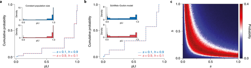
(A & B) Different combinations of h and s with the same hs value yield highly similar distributions of pLI. We considered PTVs arising in a hypothetical human gene of typical length for (A) a population of constant size and (B) a plausible model of changes in the effective population size of Europeans over time⁴⁷. We modeled the distinct number of segregating PTVs in a population using forward simulations (see Supplementary Note for details). We first obtained the number of PTVs expected under neutrality by averaging over 10⁶ simulations with s=h=0. Then, for different combinations of s and h, we calculated the pLI value for each replicate from the number of PTVs obtained. The lines show the cumulative distribution of pLI in 10⁶ replicates for the parameter combinations of s=0.1,h=0.9 (blue, dashed) and s=0.9,h=0.1 (red, solid). The insets in each figure show the density of the distribution of pLI scores. (C) The probability of observing a specific PTV count is maximized along a ridge of fixed hs. We generated the distribution of PTV counts in a hypothetical human gene under the Schiffels-Durbin model as above for a grid of s and h values, using 10⁶ replicates for each parameter combination. The figure depicts the likelihood of observing a PTV count of 3 (the value that by chance was obtained in the first run of s=0.10,h=0.90 and was treated as observed) for each combination of h and s.