Figure 7.

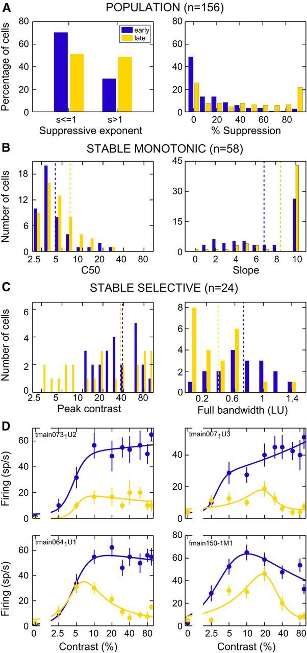
Changes in the shape of CRFs, early versus late windows. A, Entire population. In the left, the binomial distribution of the suppressive parameter (s) of well fitted neurons is shown separately for the early (in blue) and late (in yellow) time windows. The right represents the percentage of suppression of each well fitted CRF. The percentage of suppression increased significantly (p ≪ 0.01, two-tailed, paired t test) from an average value of 16 to 38%. B, Stably monotonic CRFs. The distributions of C₅₀ (left) and slope (right) for the population of stably monotonic CRFs (s ≤ 1.1) is shown, separately for the early and late windows (conventions as in A). The blue and yellow vertical dotted lines represent the average C₅₀ and slope for the early and late windows, respectively. C₅₀ did not change significantly (p = 0.16, two-tailed, paired t test), whereas the slope increased significantly (p ≪ 0.01, two-tailed, paired t test). C, Stably selective cells. The distributions of peak contrast (left) and bandwidth (right) for the population of stably selective cells (s > 1.1) is shown, separately for the early and late windows (conventions as in A). Peak contrast did not change significantly (p = 0.72, two-tailed, paired t test), whereas the bandwidth was significantly reduced in the later window (p ≪ 0.01, two-tailed, paired t test). D, Single-cell examples. Responses of four representative V4 neurons to bars of different contrast are shown. Mean firing rate [spikes per second (sp/s)] is plotted as a function of percentage Michelson contrast for the early (in blue) and late (in yellow) windows, along with the best fitted curve provided by the Peirce function (solid lines).