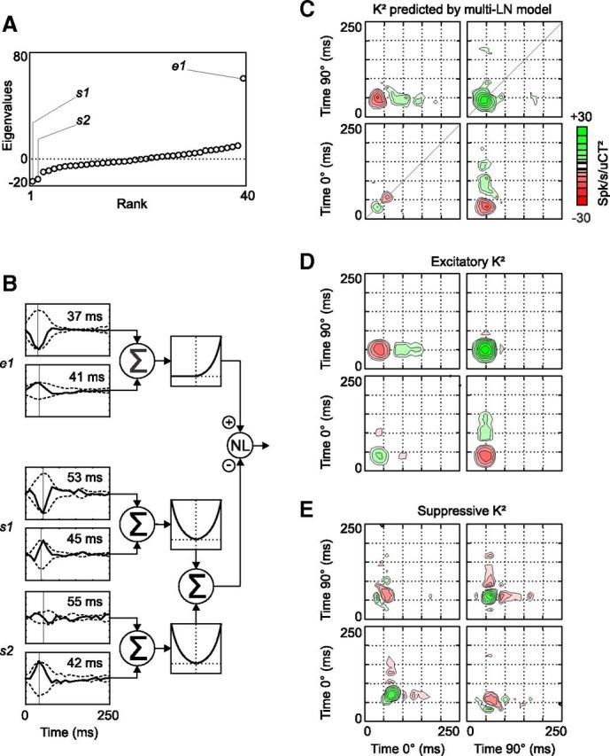
Figure 3.

The multi-LN model and its predicted K² at Hi CT (cell 1). A, Graph of the eigenvalues obtained after eigen decomposition of the K² shown in Figure 1E. Three eigenvalues (two negative and one positive) differed significantly from the eigenvalues obtained after randomly time shifting the spike responses relative to the stimulus. B, Schematic illustration of the multi-LN model of cell 1. The linear filters s₁, s₂, and e₁ each consist of two 1D filters. Their envelopes are shown (dotted lines) and the peak latency of each envelope is indicated in inset. The output of e₁ is passed to a half-squaring function, whereas the outputs of s₁ and s₂ are squared. The resulting excitatory and suppressive inputs are combined by a sigmoid nonlinearity (see Materials and Methods), which produces the response prediction. C, K² reconstructed from the response predicted by the multi-LN model in B. D, K² reconstructed from the predicted excitation (i.e., the output of the branch consisting of e₁ followed by the half-squaring nonlinearity). E, K² reconstructed from the predicted suppression, the sum of the squared outputs of s₁ and s₂. This signal then contributes to the subtractive and divisive terms of the output nonlinearity of the multi-LN model. Note that because this suppressive K² is computed before the intervention of the output nonlinearity, green regions in E correspond to interactions that suppress the final predicted firing rate, and red regions facilitate the predicted response. Note also that the diagonal interactions peak at slightly later time in E than in D.