Non-parametric group-level statistics for source-resolved ERP analysis

Abstract

We have developed a new statistical framework for group-level event-related potential (ERP) analysis in EEGLAB. The framework calculates the variance of scalp channel signals accounted for by the activity of homogeneous clusters of sources found by independent component analysis (ICA). When ICA data decomposition is performed on each subject's data separately, functionally equivalent ICs can be grouped into EEGLAB clusters. Here, we report a new addition (statPvaf) to the EEGLAB plug-in std_envtopo to enable inferential statistics on main effects and interactions in event related potentials (ERPs) of independent component (IC) processes at the group level. We demonstrate the use of the updated plug-in on simulated and actual EEG data.

I. Introduction

Independent component analysis (ICA) has been used in EEG analysis since 1996 [1]. ICA can be understood as a process of maximizing non-Gaussianity. The motivation for its application to EEG data is as follows: scalp-recorded EEG signals sums volume-conducted projections of effective brain sources, each typically indexing synchronous electrical activity across a cm-scale cortical patch and of non-brain sources (from scalp muscles, heart, eye movements and eye blinks, sweating, as well as external non-physiological noise sources). The recorded data signals are linear mixtures of these independent activities. By the central limit theorem, such a mixture approaches a Gaussian distribution. However, typically Gaussian distributions arise only from mixing, while the brain source signals of interest are non-Gaussian [2][3]. Empirical evidence has shown that mutual information reduction by ICA is associated with returning components with near-dipolar scalp maps [4].

Using ICA results, we can ask what contribution is made to the scalp EEG signals by selected brain ICs and by clusters of similar ICs found in some or all subjects. The function std_envtopo in EEGLAB quantifies the source contribution to the scalp signals in terms of percent variance accounted for (pvaf). For a given IC cluster,

$$\text{pvaf}=100-100\ast V_{\text{remainingClusters}}/V_{\text{allClusters}}$$ (1)

Here, V_{remainingClusters} is the mean of variances across summed projections of all other clusters, and V_allClusters is the mean of variances across the summed projections of all clusters.

However, there has been no statistical framework to test the significance of the pvaf measure or its group/condition differences and interactions. Part of the reason is the sub-additivity of signal variance, var(A+B) < var(A) + var(B). We have therefore developed a new statistical framework for measuring and comparing the pvaf's of IC clusters in an EEG STUDY (in EEGLAB, a grouping of comparable EEG data sets for use in comparative analysis). The purpose of the framework is to compute the statistics of differences in source IC contributions to the scalp data at the group level. We apply it here to event-related potential (ERP) averages of short data epochs time-locked to some class of experimental events of interest.

II. Methods

A. Data processing in EEGLAB: std_envtopo and statPvaf

1) IC clustering in an EEGLAB STUDY

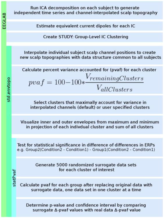
Fig. 1 shows the major processes involved in obtaining pvaf statistics. After EEG data collected from a group of subjects are preprocessed, ICA decomposition is performed on each subject's data to separate brain and non-brain source activities linearly mixed at scalp sensors. Identified ICs have maximally independent activity time series and fixed scalp topographies or maps [1]. Next, each independent component scalp map is fit to the scalp projection of an equivalent current dipole using DIPFIT 2.3 (an EEGLAB plug-in using Fieldtrip toolbox functions) [4]. IC clusters can then be created for the EEGLAB STUDY by grouping similar ICs based on similarities in equivalent dipole locations, scalp maps, mean log power spectra, event related potentials (ERPs), etc. [5].

Figure 1.

Pipeline of major processes in toolbox EEGLAB, plug-in std_envtopo, and sub-function statPvaf.

2) Envelope and topography plotting: std_envtopo

The main purpose of the std_envtopo function is to plot the envelopes of the summed scalp projections of selected IC clusters overlaid by the envelopes of scalp projection and the summed scalp maps of the largest-contributing IC clusters. Scalp recorded data (X) are modeled by

$$X=W^{-1}S,$$ (2)

where W⁻¹ is the inverse of the ICA unmixing matrix and S is the matrix of source activities. If the number of ICA components is less than number of data channels, W⁻¹ is the pseudo-inverse weight matrix. At the STUDY level, scalp projections are calculated by convolving W⁻¹ with non-artifactual component S. Because subjects may have had differing numbers of channels entered into the analysis, comparable scalp topographies for each IC are generated by interpolating the individual subject scalp map channel positions using Matlab (The MathWorks Inc., Natick, MA) function griddata.

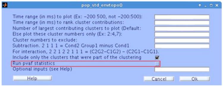
Fig. 2 shows the user interface of the std_envtopo plug-in as called from EEGLAB. The default option is to generate output for each STUDY variable combination (Fig. 3ii), but a main or interaction effect difference can be computed instead (Fig. 3iii). In the graphical output (Fig. 3i, 3ii, 4iii), black outer traces show the maximum and minimum channel values at each ERP latency, and coloured traces show the maximal and minimal projected channel values for the most strongly-contributing IC clusters; straight lines match cluster envelopes to their respective cluster scalp maps, labels, and sorting variable values; dashed vertical lines indicate the latency range in which the cluster projections are ranked.

Figure 2.

std_envtopo user interface. The default option for statPvaf is off.

Figure 3.

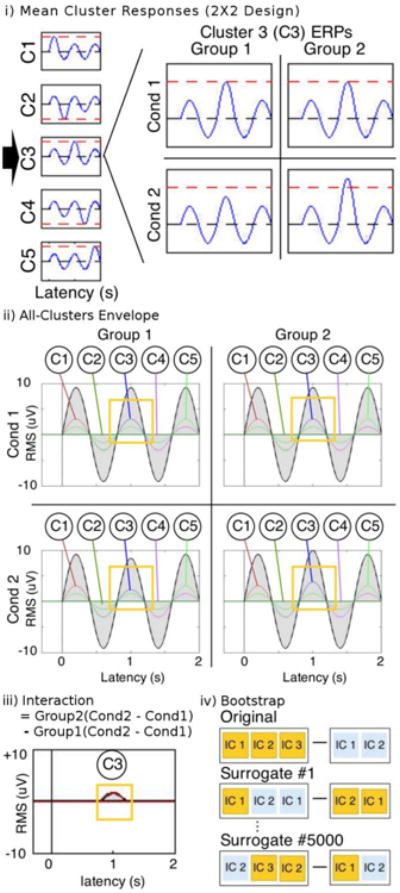
STUDY design and std_envtopo for simulated data. i) Mean cluster responses. The mean response of each cluster is a 1.25Hz sine wave with amplitude of 1, except for a specified half cycle where the amplitude is doubled. Clusters 1, 2, 4, and 5 are composed of identical ERPs in all four group-condition combinations, but Cluster 3 is composed of differing ERPs: for Condition2, the maximum amplitude is smaller in Group1 and larger in Group2. ii) Envelope plots for all group-condition combinations. The golden boxes highlight the latencies for which Cluster 3 is different. iii) Interaction envelope plot showing the difference of differences. The golden box highlights the expected contribution from Cluster 3. iv) Schematic of surrogate data generation in bootstrapping. Difference in background colours represent a difference in one STUDY variable. Note that ICs are chosen with replacement by definition of bootstrapping.

Figure 4.

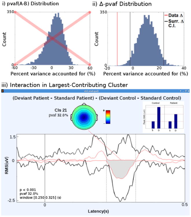
std_envtopo and statPvaf for actual data. i) Histogram of surrogate pvaf(A-B) distribution. Non-Gaussianity suggests failure in bootstrapping. ii) Histogram of surrogate Δ-pvaf (pvaf(A) – pvaf(B)) distribution. The black lines indicate the confidence interval and the red line marks the data δ-pvaf (-12.4%). iii) std_envtopo and statPvaf result Between 0.250 and 0.325s, the interaction in the Midcingulate cluster is statistically significant and accounts for 32.0% of the variance in scalp projection differences. The inset shows the 2 × 2 design. Peak in Deviant (d) condition in Control group is largest, followed by Deviant in Patient group, and finally by Standard (s) condition in both Control and Patient groups.

3) Bootstrap statistics in statPvaf

When a main effect subtraction or an interaction is specified in std_envtopo, the statPvaf sub-function can be run to perform inferential statistics on pvaf. We explain statPvaf by examining an effect of between-group conditions, namely Group1 Condition1 –Group2 Condition1 for a STUDY with a 2×2 design. First, an IC stack is created by combining ICs depending on the STUDY variable of interest; for our between-group difference, the common variable is Condition. In each of the 5,000 iterations of bootstrapping for each cluster of interest, a surrogate IC set is generated by random combination of ICs from the IC stack. The surrogate IC set is then used to calculate surrogate projections. Fig. 3iv shows a schematic for surrogate generation: in our example case, the golden boxes represent ICs from Group1 while the light blue boxes represent those from Group2. In the original data, the difference is between 3 Group1 ICs and 2 Group2 ICs; in the surrogate data, the Group variable is ignored and the difference is between any 3 Condition1 ICs and any other 2 Condition1 ICs. By randomly selecting ICs in this way, we can test the null hypothesis of statistical insignificance in Group differences.

There are two ways to statistically test pvaf in the case of a main effect subtraction. One method is to first calculate pvaf(A) from one set of projections and pvaf(B) from another, then create a distribution of the difference pvaf(A) – pvaf(B). The other method is to calculate pvaf(A – B), the pvaf in the grand projection difference. We adopted the first method instead of the second because the surrogate distribution of the former was closer to Gaussian (Fig. 4ii) while the distribution of the latter was skewed (Fig. 4i). Due to the central limit) theorem, the difference of the surrogate values should converge towards a Gaussian distribution. The following example shows one reason why distributions obtained from the two methods differ in normality. In an extreme case of bootstrapping where surrogate Group1 ICs are completely replaced by the original Group2 ICs and vice versa, the projection difference retains its magnitude and changes polarity. The variance remains the same, and the original data pvaf(A – B) is equivalent to surrogate pvaf(B – A). When pvaf is calculated from each projection instead of the projection difference, the surrogate pvaf(B) – pvaf(A) is equal in magnitude and opposite in polarity to the original data's pvaf(A) – pvaf(B). If only half the ICs are bootstrapped and each surrogate data set retains at least half of its original ICs, the distribution of pvaf(A – B) is close to Gaussian (data not shown). Therefore, we define Δ-pvaf as pvaf(A) – pvaf(B) and use its distribution as input to statistics functions stat surrogate_pvals and stat surrogate_ci (EEGLAB functions developed by Tim Mullen, SCCN) to calculate empirical p-values and confidence intervals.

statPvaf can also be used when exploring 2 × 2 interaction such as (Group2 Condition2 - Group2 Condition1) – (Group1 Condition – Group1 Condition1). Two IC stacks are formed per cluster, and two surrogate IC sets are generated per iteration. To test the null hypothesis of statistical insignificance for group IC differences, bootstrapping generates a surrogate set which has IC randomization between Group2 Condition1 and Group1 Condition1 and between Group2 Condition2 and Group1 Condition2. A pvaf value is calculated for each group by applying (1) on each of the two within-group projection differences; for example, Group2 pvaf is calculated on Group2 Condition2 – Group2 Condition1. In this particular STUDY interaction, Δ-pvaf is the difference of Group 2 pvaf and Group1 pvaf.

B. Simulated STUDY with 2 × 2 Design

A simulated EEGLAB STUDY was created to test std_envtopo. The STUDY features a 2 × 2 design with 20 subjects, each with 20 ICs. The subjects were divided between Group1 and Group2 (ten subjects per group), and each subject's ICs were divided between Condition1 and Condition2 (ten ICs per condition). The 400 total ICs were separated into 5 clusters (80 ICs per cluster), and all clusters were assigned the same scalp topography to prevent differences in projection. Clusters 1, 2, 4, and 5 are composed of identical ICs in all four group-condition combinations, but Cluster 3 is composed of differing ICs (Fig. 3i).

To confirm the structure of the STUDY design, we first used std_envtopo to create plots for each group-condition combination. Then, with the same latency window, we plotted the largest contributing cluster in the interaction of condition × group, namely (Group2 Condition2 – Group2 Condition1) – (Group1 Condition2 – Group1 Condition1).

In this simulation, it is predicted by definition that the pvaf of Cluster 3 in the difference ERP will always be 100% because the contribution of all other clusters are simulated to be exactly zero after subtraction, regardless of how the ICs are shuffled and projections are subtracted. The parameters are shown in Table I.

Table I. Std_Envtopo Parameters.

Parameters	Data Set
	Simulation	Actual
Time range (in ms) to plot:	[-300 2000]	[-200 500]
Time range (in ms) to rank cluster contributions:	[0 2000]	[220 325]
Number of largest-contributing clusters to plot	5	1
Factorial Design	2 × 2 Interaction	2 × 2 Interaction
Number of clusters used in statPvaf	1	1

C. Application to Actual STUDY with 2 × 2 Design

The duration mismatch negativity task was performed on 42 non-psychiatric subjects (NCS) and 47 schizophrenia patients (SZ) [6]. The factorial design of the experiment was 2 × 2 mixed design; stimulus types (Standard, Deviant) as a within-subject condition vs. group as a between-subject condition. std_envtopo and statPvaf were applied to examine the interaction of stimulus types by group, namely (Deviant Patient – Standard Patient) – (Deviant Control – Standard Control). The parameters are shown in Table I.

III. Results

Fig. 3 shows the std_envtopo results for the simulated study. The envelope plots for all Group-Condition combinations in Fig. 3ii show the latencies at which each cluster has maximum contribution. We omitted the scalp maps since they were simulated to be consistent across all clusters. As expected, Cluster 3 accounted for 100% of the variance in the interaction of condition × group (Fig. 3iii). Δ-pvaf is 0%. In the envelope plots for all group-condition combinations, Clusters 1 through 5 showed maximal contribution during their respective half cycle, and both the inner and outer envelopes in the 3^rd half cycle reflect the influence of Cluster 3's unique ERP design. In the envelope plot of the interaction, there is no signal except for the latency corresponding to the 3^rd half cycle of the sine wave. Since this latency window corresponds to Cluster 3, the plot and the calculated pvaf value match the expectation that only Cluster 3 would have a nonzero interaction term and account for all of the variance in the interaction.

Fig. 4 shows std_envtopo results for the STUDY. Fig. 4i gives schematics of the interaction in the 2 × 2 STUDY. The interaction term contribution of the Mid-Cingulate cluster was the largest with a pvaf of 32%. The histogram in Fig. 4ii shows the distribution of surrogate Δ-pvaf values, ranging from -18% to 36%. In line with the central limit theorem, the surrogate Δ-pvaf distribution approaches a Gaussian form. The upper and lower bounds of the confidence interval were 23% and -2% respectively. In the original data, pvaf was 10% and 22% in Patient and Control group respectively, giving a Δ pvaf of -12%. This difference reached statistical significance at p<0.001 (Fig. 4iii).

IV. Discussion

We demonstrated how std_envtopo and stdPvaf work using simulated and actual data. We also compared the two approaches to construct surrogate data, namely pvaf(A - B) and pvaf(A) - pvaf(B) (i.e. Δ pvaf), and showed that Δ pvaf is preferable since it has a Gaussian distribution. It should also be noted that this is the first dedicated explanation of the std_envtopo function used in EEGLAB. Its significance is to bridge the ‘projected’ scalp channel measures to the underlying source-resolved brain EEG activities by computing the accounted variance of the latter in the former. The methods presented address a previously unmet need to perform inferential statistics on pvaf, a measure useful for determining which IC clusters to analyze. The addition of statPvaf to std_envtopo may further encourage and facilitate the use of ICA for EEG analysis. In future, statistical methods of multiple comparison correction such as the Bonferroni-Holm method will be incorporated to refine multi-cluster statPvaf. The user interface of std_envtopo will also be improved to allow more intuitive option selection.

V. Conclusion

Functions std_envtopo and statPvaf enable us to ask how much ERP variance is accounted for by source-resolved EEG activities, to identify largest-contributing IC clusters, and to determine whether their contributions are significantly different across conditions. They connect effective EEG sources to their scalp projections by showing the contribution of the former to the latter.

References

- 1.Makeig S, Bell A, Jung T, Sejnowski T. Indepdent component analysis of Electroencephalographic data. Advances in Neural Information Processing Systems. 1996;8:145–151. [Google Scholar]
- 2.Friston K. Modes or models: a critique on independent component analysis for fMRI. Trends in Cognitive Sciences. 1998;2(10):373–375. doi: 10.1016/s1364-6613(98)01227-3. [DOI] [PubMed] [Google Scholar]
- 3.Onton J, Westerfield M, Townsend J, Makeig S. Imaging human EEG dynamics using independent component analysis. Neuroscience & Biobehavioral Reviews. 2006;30(6):808–822. doi: 10.1016/j.neubiorev.2006.06.007. [DOI] [PubMed] [Google Scholar]
- 4.Delorme A, Palmer J, Onton J, Oostenveld R, Makeig S. Independent EEG Sources Are Dipolar. PLoS ONE. 2012;7(2):e30135. doi: 10.1371/journal.pone.0030135. [DOI] [PMC free article] [PubMed] [Google Scholar]
- 5.Delorme A, Mullen T, Kothe C, Akalin Acar Z, Bigdely-Shamlo N, Vankov A, Makeig S. EEGLAB, SIFT, NFT, BCILAB, and ERICA: New Tools for Advanced EEG Processing. Computational Intelligence and Neuroscience. 2011;2011:1–12. doi: 10.1155/2011/130714. [DOI] [PMC free article] [PubMed] [Google Scholar]
- 6.Rissling A, Miyakoshi M, Sugar C, Braff D, Makeig S, Light G. Cortical substrates and functional correlates of auditory deviance processing deficits in schizophrenia. NeuroImage: Clinical. 2014;6:424–437. doi: 10.1016/j.nicl.2014.09.006. [DOI] [PMC free article] [PubMed] [Google Scholar]